More Scraping + Crosstalk

Recently, I had become curious of what more I could do with the Rvest package. I knew that I could rip elements and tables from off of websites, but I wanted to see what else I could do. I know that there are better scraping techniques, but I wanted to become more proficient at grabbing useful information and tabulating them. Today, I want to show you a recent project I finished on how to automate a data collection process for select interest variables! Afterwards, I’ll display the information through Crosstalk. A useful HTML widgets package. I guess I won’t be going into creating any deliverables for website integration, but just putting information side by side for easier data representation.

Here we go.

At the beginning, I wasn’t sure what to do. My first thought was to begin with a google search function. I thought that would be a good way to start. I knew that anything that came after…

  ## "https://www.google.co.in/search?q="

stood for a search term with “+” in between the spaces. I then decided that I wanted to find all the top web links associated with each search term. So, I expanded on this idea and cleaned up a bit of code to make myself a function that extracted only the urls that appeared on the page.

Glinks <- function(x) {
  require("rvest")
  # create url
  srch <- "https://www.google.co.in/search?q="
  term <- sub(" ","+",x)
  term <- paste(srch,term, sep = "")
  hh <- term %>% read_html()
  # Find location
  links <- hh %>% 
    html_nodes(xpath='//h3/a') %>% 
    html_attr('href')
  # extract URL
  gg <- grep('url',links) %>% as.vector()
  crowl <- links[gg] %>%
    strsplit(split='&') %>%
    sapply('[',1)
  # Output
  gsub('/url\\?q=','', crowl)
}

This actually didn’t take so long. Now I had a function that printed a vector of many weblinks. Yet, it seemed a little too useless at the moment. Maybe a fun party trick for those that don’t know how to code things up? I knew there was more I could do. Look up your name or anything and you can see that the google search that comes up will be the same as the weblinks that show up.

Glinks("Pluralsight")

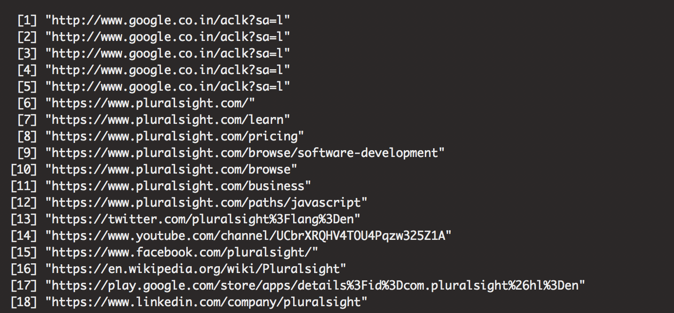
You can see how the links associated with this page displays all types of links shown on the main page. I guess I could tweak it a bit, so it pulls up links from the top box on the right, but I will look at that later.

I decided from there that I wanted to choose an industry, look up some companies, and pull information from the internet. I also wanted this to be something that can be automated across a specific industry, so if I ever came to a point in time where I needed to do any industry-specific research, I could compile meaningful data.

Just on a whim, I decided on the auto industry just for fun. I picked 10 companies just randomly and decided that I needed to scrape uniform information to prepare for any type of analysis. Unfortunately, the only place I could find similar information across all links was the main page of the car company or the Wikipedia page. Just for sake of easier automation, I decided on looking up uniform information from car companies!

After picking these car companies, I replicated the Glinks function over the vector of names and picked only the Wikipedia articles

# Let's just say I am only interested in 10 car companies
Glinks("Hyndai Motors")
names <- c("Chrysler","BMW","Ford","Tesla", "Toyota",
           "Volkswagen Group","Hyundai Motors","Nissan","GM","Honda Motors")
# search links based on name.
srch <- sapply(names,Glinks)

# extract only wikipedia 
wikis <- c()
for ( i in 1:length(names)) {
 wikis[i] <- srch[[i]][grepl("en.wikipedia.org",srch[[i]])][1]
}
cars1 <- data.frame(names,wikis)
cars1

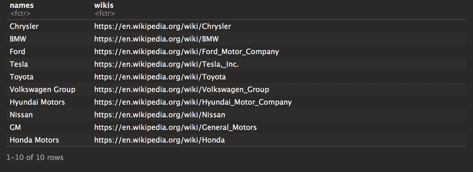
It looks nicely compiled! Now I revisited one of the rvest posts that I wrote a while back and extracted the main table that supplies the information I need. You can take a look at it here. I looked to table the important information. During the process, I realized that Nissan had an extra table that made the xpath the 2nd table in the page. I guess if the Wikipedia page changes, it will revert back to the top. I should keep that in mind when revisiting this specific scraping method for information.

cc <- list()
for (i in 1:nrow(cars1)) {
  if (cars1[i,1]!="Nissan") xp <- '//*[@id="mw-content-text"]/div/table[1]'
  else xp <- '//*[@id="mw-content-text"]/div/table[2]'
  path <- cars1[i,2] %>% as.character()
  cartab <- path %>%
    read_html() %>%
    html_nodes(xpath = xp) %>%
    html_table()
  cc[[i]] <- cartab[[1]]
}

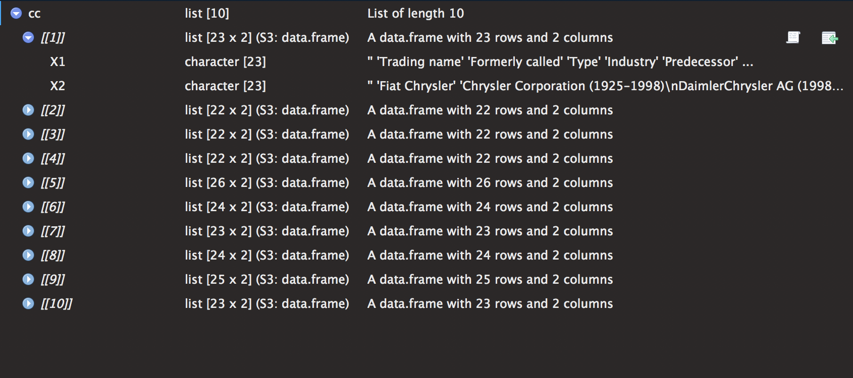
The list cc has 10 elements with a table of dimensions 2 X 22. I then proceeded to create the variables of interest (using more regex, just for fun). There is definitely a quicker and easier way to create the columns, but I guess I just wanted to do something fun. I then took elements of list and used the do.call() function. Very useful when trying to perform any function over a list.

# create columns
pattern <- "Revenue|Operating income|Net income|Total assets|Total equity|Number of employees"
coln <- gsub("\\|",",",pattern)
coln <- c("Names","wikis",strsplit(coln,",")[[1]])
# Fill columns
car.data <- list()
for (j in 1:nrow(cars1)) {
  create <- cc[[j]][pattern %>% grepl(cc[[j]][,1]),2] %>% t()
  create <- as.data.frame(create)
  car.data[[j]] <- cbind(cars1[j,],create) 
}
car.datas <- do.call("rbind",car.data)
colnames(car.datas) <- coln
glimpse(car.datas)

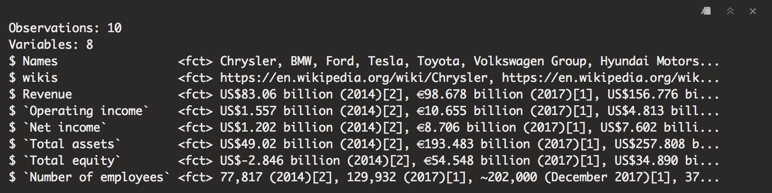
Now I have a table with a bunch of information I need to perform an analysis. Now we run into the problem of having to clean out information. With lots of unimportant boxes, units, and currencies it can get a little hairy with creating useful and expansive information. We’ll proceed to clean the info and make it useful for anyone that needs it!

# function to rid of junk.
annoying <- function(x) {
  x <- gsub("\\[.*?]","",x)
  x <- gsub(" \\(.*?)","",x)
  x <- gsub(",","",x)
  x <- gsub("KRW ","W",x)
  x <- gsub("\\$ ","$",x)
  x <- gsub("US","",x)
  gsub("~","",x)
}

# sapply annoying
car.datas <- sapply(car.datas, function(x) annoying(x))
car.datas <- data.frame(car.datas) # re-coerce as a data.frame

# separate units (trillion/billion)
indicator <- colnames(car.datas)[-c(1:2,8)]
for (i in 1:length(indicator)) {
car.datas <- car.datas %>% 
  separate(indicator[i], c(indicator[i], "Units"), sep = "\\s+")
}

Once again, I brought up the same function used in my credit card analysis and did a similar function to rid the useless info. Unfortunately, this time around the cleaning is not as easy as we would like it. After cleaning the junk, I needed to make sure to separate the units, so I can revisit and create uniform numbers across the dataset. To do this, I used a similar technique as when I split the date information for the Poisson post.

Now that the units had been extracted, I set out to clean some more. Yet, this time I proceeded to grab all the currency information, from yahoo in the quantmod library. This is a useful tool that update stock information, currency exchange, and any other financial information that needs to be quickly updated. I’ll probably explore this more in the future.

Afterwards, we can create two new variables “Currency” and “FX”. Once this is done, we can safely remove all of the currency signs to start some computations.

# Quick look up currency
library(quantmod)
from <- c("EUR", "JPY","KRW")
to <- c("USD","USD","USD")
curr <- getQuote(paste0(from, to, "=X"))[,2]

# Extract currency values
for (i in 1:nrow(car.datas)) {
  if (grepl("\\$",car.datas$Revenue[i])) {
    car.datas$Currency[i] <- "Dollars" 
    car.datas$FX[i] <- 1
    }
  else if (grepl("\\€",car.datas$Revenue[i])) {
    car.datas$Currency[i] <- "Euros" 
    car.datas$FX[i] <- curr[1]
    }
  else if (grepl("\\¥",car.datas$Revenue[i])) {
    car.datas$Currency[i] <- "Yen" 
    car.datas$FX[i] <- curr[2]
    }
  else if (grepl("\\W",car.datas$Revenue[i])) {
    car.datas$Currency[i] <- "Won"   
    car.datas$FX[i] <- curr[3]
    }
}

# Remove signs
sign.removal <- function(x) {
  x <- gsub("\\$","",x)
  x <- gsub("\\€","",x)
  x <- gsub("\\¥","",x)
  gsub("W","",x)
}
car.datas <- sapply(car.datas, function(x) sign.removal(x))
car.datas <- data.frame(car.datas)

Following this, we can finish by changing the classes of the columns, creating a new frame that uses only dollars, and standardizing the units to all billions. This was done simply by some nested for loops that took each information and modified it to our liking.

# Change columns of interest to numeric
for (i in c(3,4,5,6,8,9,11)) {
  car.datas[,i] <- as.numeric(as.character(car.datas[,i]))
}


car.datas.dol <- car.datas
for (j in 1:nrow(car.datas)) {
  for (i in c(3,4,5,6,8)) {
    car.datas.dol[j,i] <- car.datas[j,i]*car.datas[j,11]
  }
}

for (i in 1:nrow(car.datas)) {
  for(j in c(3,4,5,6,8)) {
    if(car.datas$Units[i]=="trillion") {
    car.datas.dol[i,j] <- car.datas.dol[i,j]*1000
    car.datas.dol$Units[i] <- "billion"
    } 
  }
}

Now take a look at our table.

car.datas.dol[,1:9]

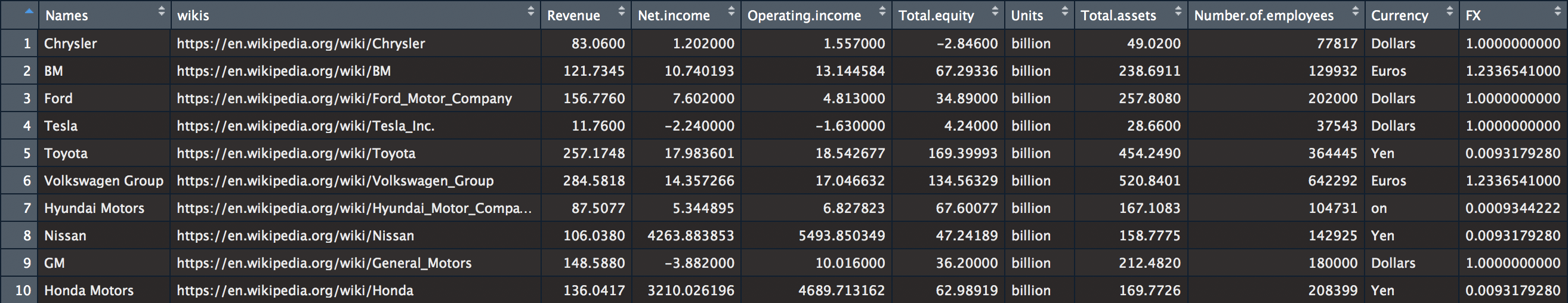
Neat huh? The table is neat and organized all without having to visit a single website! Let’s now make a pretty graphic to show summary statistics.

Crosstalk is kind of like an add-in for plotly or for shiny that lets you create better interactive visuals. For example, if we were looking to create a side-by side visual for revenue, but from operating income and total equity, you could do this rather easily. I have no need for this data, nor do I think it tells anything important other than the size of the company, but I just want to show you for interpretation sake.

library(crosstalk)
# define a shared data object
d <- SharedData$new(car.datas.dol)
# make a scatterplot of disp vs mpg
ogscatterplot <- plot_ly(d, x = ~`Total.assets`, y = ~Revenue) %>%
  add_markers(color = I("navy"))
# define two subplots: boxplot and scatterplot
subplot(
  # boxplot of disp
  plot_ly(d, y = ~Revenue) %>% 
    add_boxplot(name = "overall", 
                color = I("navy")),
  ogscatterplot, 
  shareY = TRUE, titleX = T) %>% 
  layout(dragmode = "select")

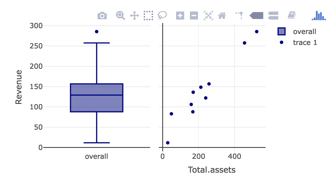
There have been several times when I wondered how to do something like this. Especially with an interactive graph. I hope you find this to be useful. I will most likely be working more with interactive plots in the future! If you are interested in checking out more about how to use plotly and simple interactive graphs, click here