Recursive partitioning is rather intuitive.

That is why it has become popular. In some cases, it is favored over other heiarchial methods. The past heiarchial methods begin with individual items and keep close items within a metric. Recursive methods start with a single cluster and divide into groups that have the smallest within cluster distances.
We must remember however, that partitioning and clustering algorithms are similar but different. Clustering deals with unsupervised learning, whereas partitioning needs labels in the data. You can view my last post on clustering here.
library(rpart)
library(rpart.plot)
library(tidyverse)
Let’s say we just want to create an intuitive diagram that shows the economics of an individual buying a car. When will he bend to make a new decision? At which level in which class will the marginal cost outweigh the quality?
We have a nice dataset from UC Irvine that will give us some help.
cn <- c("price","maint","doors","persons","luggage","safety","acceptable")
dat <- read_csv("https://archive.ics.uci.edu/ml/machine-learning-databases/car/car.data",col_names = cn)
dat <- drop_na(dat)
## buying: vhigh, high, med, low.
## maint: vhigh, high, med, low.
## doors: 2, 3, 4, 5more.
## persons: 2, 4, more.
## lug_boot: small, med, big.
## safety: low, med, high.
## acceptable: acc, good, unacc, vgood
The structure of the data is rather intuitive (and clean!). Our goal now is to map how acceptable a car is given some quality. It’s really easy (as long as we are not looking to evaluate our model..). We really don’t need to for this specific example, but we will create our own train and test sets.
set.seed(15)
train.ind <- sample(nrow(dat),nrow(dat)*.80)
train.dat <- dat[train.ind,]
test.dat <- dat[-train.ind,]
We notice though, that the data is so small, some of the information will get lost in our train set (5184 possible variations where we only have 1728 rows of data). Good thing we are only mapping the information for our eyes.
Let’s go ahead and fit a decision tree by classification
train.fit <- rpart(acceptable~ ., data = train.dat, method = "class")
We must specify class here as every column is made up of factors. Other than that, it’s real simple. Our output/diagram will be given below.
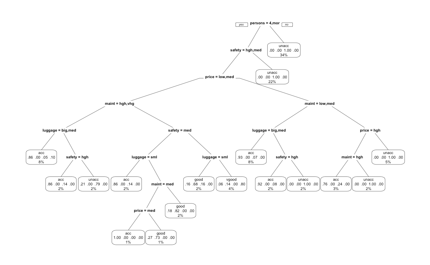
rpart.plot(train.fit, extra = 104, trace = 1) # specify 104 for multiple classes..

Unfortunately, it’s really small. Even after tweaking the plot cex and limits, we notice how the graphics are insufficient. Hopefully, this feature will be added on in the future.
Alternatively, if we’re not looking for something too rigorous, we have this.
prp(fit,extra = 104)

We notice how intuitive this diagram is. Most people look for 4 person seats with high to medium safety. Depending on the price, we would naturally seek to optimize the maintenance and luggage space. It is also interesting to note the heiarchy of importance as seats, safety, and price are amongst the highest nodes. We also notice how some of these parameters are recursive as safety, price, and maintenance appears in multiple locations from top to bottom.
For a numeric dataset, we would evaluate the model by predicting our values and identifying the lowest root mean sum of squared errors as below:
rpart_test_pred <- predict(test.fit,test.dat[,-7],type = "vector" )

#calculate RMS error IF numeric..
rmse <- sqrt(mean((rpart_test_pred-test.dat$acceptable)^2)) # this will give us an error.
For classification, we should be looking at precision, accuracy, and F1 scores. The higher the better. However, we will not be going through too much model evaluation because this dataset is small and intuitive. Model evaluation will be necessary when moving away from recursive partitioning and into more complex decision trees. If you’re interested in class-based classification metrics, take a look at the clustering algorithms post specified at the beginning.
If you are interested, some other “tree”-based algorithms ( random forest and phylogenetic trees) they are all in the archive.