How well do you usually sleep? The average adult gets about 7-9 hours of sleep. Does that feel like enough to you?

Today, we will classify good and bad sleep using a beta-binomial bayesian inference. We will, step by step, work through how to update our priors and create new posterior distribution.
This analysis will need a bit of bayesian intuition, so if you want to read up on what we are doing, click here. If you are further confused, send me a message and I will get right back to you.
Let’s get started. How often do we get “good” sleep?
We’ll take our friend Bob here. He feels like he gets about 7-8 hours of sleep on average, quite the average sleeper. We want to figure out here how likely is it that he is getting good sleep?
For this task, we will use the beta-binomial distribution as we need a conjugate prior to the success-failure nature of the question: “Is he getting good enough sleep?” Let’s define what we are measuring and considerit a success when we have had at least 7 hours of sleep and a sleep quality over 60% (sounds reasonable doesn’t it?). Sleep is measured in hours and quality is measured by how efficient (deepness and within cycle) we are sleeping. It’s easy to judge how long we are sleeping, but a bit difficult to measure how well we are sleeping. Under those standareds Bob feels like he gets a good amount of sleep about 6/10 of his nights with quite some certainty.
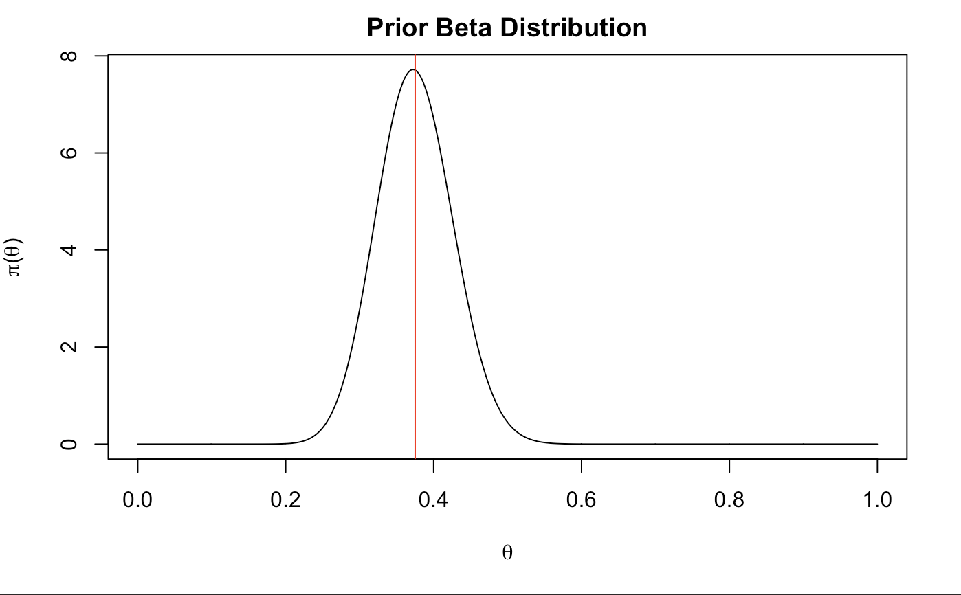
Let’s create our prior! Since we are working with binomial data, we will measure a beta distribution of our guess (it is a conjugate with the same kernel). In the easiest of explanations, alpha corresponds with the amount of successes and beta corresponds to the frequency of failures. If 6/10 times we succeed in sleep, alpha could be a big bigger than half of beta. Let’s choose beta to be 55 and alpha to be 33. The larger alpha and beta are (from 0 to infinity) the more certain we are of our guesses.
# 55*6/10 = a
a <- 33
b <- 55

xx <- seq(0,1,length.out = 1000)
prior <-dbeta(xx,a,b)
plot(xx,prior,type="l", main="Prior Beta Distribution",xlab=expression(theta),
     ylab= expression(paste(pi, "(", theta, ")", sep="")))
(beta_mean <- mean(replicate(1000,mean(rbeta(1000,a,b))))) # Monte carlo mean.
abline(col = "red", v = beta_mean)

## [1] 0.375042
That looks about just right. We are centered at about .4 which shows that we have just a little less good sleep than bad sleep just around half. It is also slightly centered to the left which shows a pretty close representation of the proportion of times we sleep well.
Now let’s collect some data on our sleep.We will be wearing some smartwatch to track our progress. The data from our smartwatch will be on my repository right here.
require(tidyverse)
path <- "https://raw.githubusercontent.com/tykiww/projectpage/master/datasets/sleep/sleepdata.csv"
raw <- read.csv(path,sep = ";", stringsAsFactors = FALSE) %>% as_tibble
glimpse(raw)
## Observations: 587
## Variables: 8
## $ Start            <chr> "2017-08-30 01:34:09", "2017-08-31 00:41:25", "2017-09-01 01:42:12", "2017-09-01 03:16:37", "2017-09-...
## $ End              <chr> "2017-08-30 08:28:12", "2017-08-31 09:18:49", "2017-09-01 02:29:06", "2017-09-01 10:30:19", "2017-09-...
## $ Sleep.quality    <chr> "63%", "78%", "10%", "69%", "88%", "100%", "76%", "86%", "96%", "62%", "86%", "77%", "59%", "75%", "6...
## $ Time.in.bed      <chr> "6:54", "8:37", "0:46", "7:13", "7:31", "10:26", "6:31", "7:40", "8:38", "6:40", "9:19", "8:09", "6:0...
## $ Wake.up          <lgl> NA, NA, NA, NA, NA, NA, NA, NA, NA, NA, NA, NA, NA, NA, NA, NA, NA, NA, NA, NA, NA, NA, NA, NA, NA, N...
## $ Sleep.Notes      <lgl> NA, NA, NA, NA, NA, NA, NA, NA, NA, NA, NA, NA, NA, NA, NA, NA, NA, NA, NA, NA, NA, NA, NA, NA, NA, N...
## $ Heart.rate       <lgl> NA, NA, NA, NA, NA, NA, NA, NA, NA, NA, NA, NA, NA, NA, NA, NA, NA, NA, NA, NA, NA, NA, NA, NA, NA, N...
## $ Activity..steps. <int> 417, 5701, 4147, 5001, 3801, 6909, 11928, 19869, 11744, 18697, 9065, 8153, 7386, 10452, 13581, 13478,...
After some cleaning, we are ready to update our new posterior distribution! The data was aggregated based on days. This may skew the data in a direction as I am assuming the same sleep hours and averaging the qualities for any duplicates (a better option may be to use a weighted average), however this should not be of too much concern.
# Cleaning
raw1 <- select(raw,Start,Sleep.quality, Time.in.bed)
raw1$Start <- as.POSIXct(raw1$Start) %>% substr(1,10)
raw1$Sleep.quality <- parse_number(raw1$Sleep.quality)/100
raw1$Time.in.bed <- raw1$Time.in.bed %>% strsplit(":") %>%
  sapply({ function(x) { x <- as.numeric(x) ; (x[1]*60+x[2])/60 } })


# Aggregation
sleep <- aggregate(raw1$Time.in.bed,by = list(raw1$Start), sum) %>%
  merge(aggregate(raw1$Sleep.quality,by = list(raw1$Start), mean), by = "Group.1")
names(sleep) <- c("date","hours","Quality")
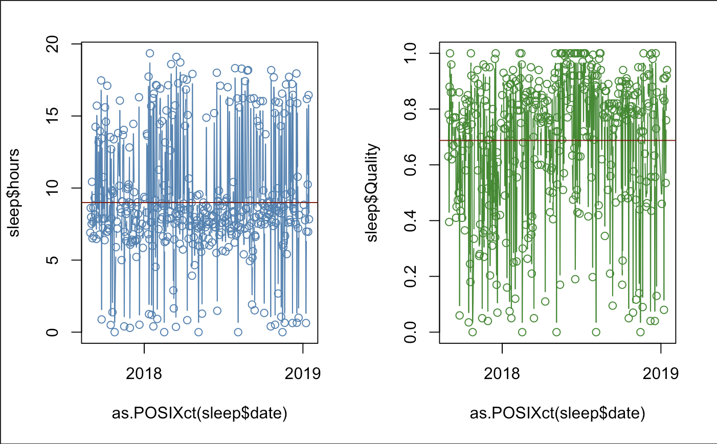
Here is a quick display of our sleep time-series.
par(mfrow=c(1,2))
plot(as.POSIXct(sleep$date),sleep$hours,type = "b", col = "steel blue")
abline(h = mean(sleep$hours), col = "dark red")
plot(as.POSIXct(sleep$date),sleep$Quality, type = "b", col = "forest green")
abline(h = mean(sleep$Quality), col = "dark red")
par(mfrow=c(1,1))

There seems to be a slight-regular pattern, but this may be for a different analysis. It is good to know that our data is not too out of place. We also notice that we seem to actually be sleeping above 60% quality. Our guess doesn’t seem so bad.
Now we will separate our data to fit a binomial distribution by making the points with at least 7 hours of sleep and a sleep quality over 60% a success.
(y <- ifelse(sleep$hours>7,TRUE,ifelse(sleep$Quality>60,TRUE,FALSE)) %>% sum)
## 295
Now we create the new distribution. Interestingly, this part isn’t too difficult for this conjugate pair. Even the math isn’t too confusing either. We take the formula and condense it into a more readable format.
\[\pi(\theta) = \frac{\binom{n}{y}\theta^y(1-\theta)^{n-y} \, \frac{\Gamma(\alpha + \beta)} {\Gamma(\alpha)\Gamma(\beta) }\theta^{\alpha-1}(1-\theta)^{\beta-1}}{\int_{0}^{\infty}\binom{n}{y}\theta^y(1-\theta)^{n-y} \, \frac{\Gamma(\alpha + \beta)}{\Gamma(\alpha)\Gamma(\beta)}\theta^{\alpha-1}(1-\theta)^{\beta-1}}\] \[New\,Distribution = \frac{(Binomial\,Likelihood\,"The\,Data")\,\,\,\,\,(Beta\,Prior\,Distribution\,"Our\,Guess")} {Total\,Probability}\]It turns out, our new posterior distribution ends up becoming a beta distribution with a new alpha and beta. Fortunately for us, it follows a unique pattern that can be followed every time!
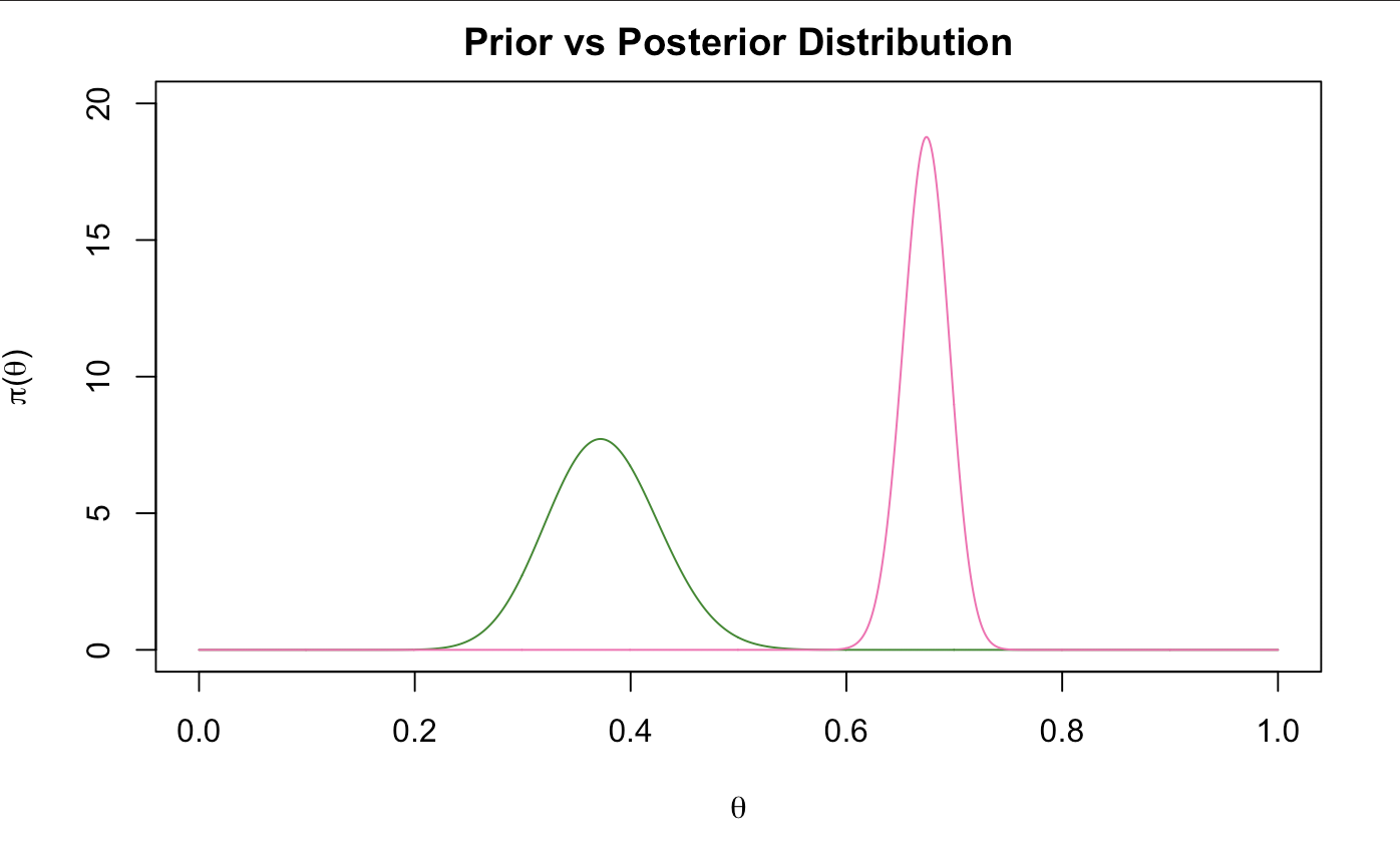
\[Prior \, \alpha = Our \,guess \\ Prior \, \beta = Our \,guess \\ Posterior \, \alpha^* = \alpha + (\#\, of \, Successes) \\ Posterior \, \beta^* = \beta + (\#\, of \, Failure)\]In our case, alpha is 33, beta is 55, # successes is 295 and our observed # failures is 104. It looks like our data outweighed our guesses. Let’s stick those into our new beta distribution.
n <- nrow(sleep)
(astar <- a + y)
(bstar <- n-y + b)
## [1] 328
## [1] 159
posterior <-dbeta(xx,astar,bstar)
plot(xx,prior,type="l", main="Prior vs Posterior Distribution",xlab=expression(theta),
     ylab= expression(paste(pi, "(", theta, ")", sep="")), ylim = c(0,20), col = "forest green")
lines(xx,posterior,type="l",xlab=expression(theta),
      ylab= expression(paste(pi, "(", theta, ")", sep="")), col = "hot pink")
c("lower" = qbeta(.025, astar, bstar), "upper" = qbeta(.975, astar, bstar))
##     lower     upper
## 0.6312536 0.7144191

We notice here that our prior beliefs were not as correct as we thought they were, however, we see from the math that it had an influence on our data with some intuitive feel of how we actually slept. Here, we can say that probability that the proportion of our sleep time is within this interval (0.6312536, 0.7144191) 95% of the time.
Now, when we make predictions, we can use the new distribution to make our guesses! The probability that we sleep at 70% efficiency more than 80% of the time is..
1-qbeta(.80,328,159)
## [1] 0.3085367
Remember now that the data we specify is not expressed in terms of confidence, rather credibility. In this way, bayesian inference is much simpler and much more intuitive than the frequentist sense. The frequentist process demands that inference cannot be made until data is collected. It looks at the probability that something happens by chance, if theoretically occuring over multiple samples that either have already happened, or have not happened yet. For them, probability is defined as the ‘proportion’ of times an event would happen in the long run.For bayesian statistics, probability is the degree of belief that a certain event would occur. It bases their inference on past data, current belief or intuition.
Next time you spot an occurance of a binomial likelihood, give this distribution a try! It’s a neat way to model our next “best” guess.