Eden Hazard is possibly the best Belgian soccer player in history. Since 2012, he has incrementally developed into a world-class star showered with FA cup and Premier league honors.
(This post was written before his trade to Real Madrid) Given his track record per season at Chelsea, let’s take a look at his goal rate using a poisson-gamma bayesian model. For this post, understanding bayesian probabilities is a prerequisite, so you may want to revisit it after learning the bayesian learning cycle. We’ll run through a complete poisson-gamma analysis of Hazard and compare him to Lampard’s time in Chelsea (league play only). Even for those not interested in soccer, this is still widely applicable for any poisson-type data.
Instead of going through and explaining the statistical distributions and their assumptions, let’s just go ahead and look at our data.
Data
Our prior belief is that Hazard, on average, would make about 1 goal every three games whereas Lampard (in his prime) would score 1 every other game. This means that we will be using a gamma distribution for our prior with shape and scale.
# Hazard Goals (Prior Beta(1,3))
h_apps <- c(34, 35,38,31,36,34,25)
h_gols <- c(9,14,14,4,16,12,12)
h_year <- 2013:2019
hazard <- data.frame("season" = h_year,"apps" = h_apps,"goals" = h_gols)
# Lampard Goals (Prior Beta(1,2))
l_apps <- c(37,38,38,38,35,37,24,37,36,24,30,29,26)
l_gols <- c(5,6,10,13,16,11,10,12,22,10,11,15,6)
l_year <- 2001:(2000+length(l_gols) )
lamprd <- data.frame("season" = l_year,"apps" = l_apps,"goals" = l_gols)
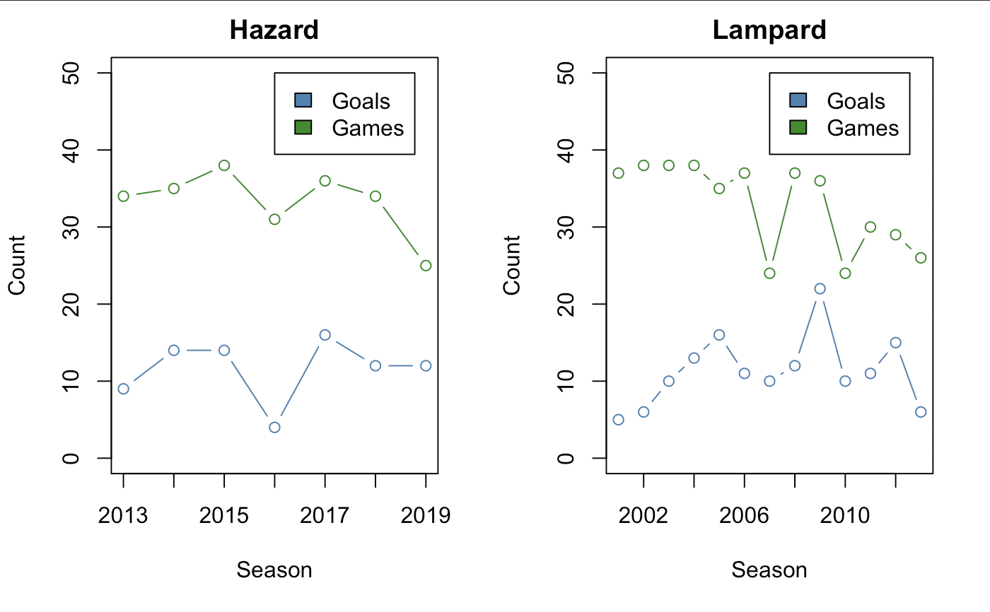
We have both the appearances and number of goals for both Hazard and Lampard. Clearly, Super Frankie Lampy is retired and has played longer, but that should not interfere with our comparison. Mapping their performance below…
par(mfrow = c(1,2))
# Hazard
plot(hazard$season,hazard$goals, type = "b", col = "steel blue",
     ylim = c(0,50), ylab = "Count", xlab = "Season", main = "Hazard")
lines(hazard$season,hazard$apps, type = "b",col =  "forest green")
legend(2016,50,c("Goals","Games"),c("Steel Blue", "Forest Green"))
# Lampard
plot(lamprd$season,lamprd$goals, type = "b", col = "steel blue",
     ylim = c(0,50), ylab = "Count", xlab = "Season", main = "Lampard")
lines(lamprd$season,lamprd$apps, type = "b",col =  "forest green")
legend(2007,50,c("Goals","Games"),c("Steel Blue", "Forest Green"))
par(mfrow = c(1,2))

Now, at this time the post is written, the 2019 season has not ended quite yet so Hazard’s current statistics are not completely up to date. However, we see a that there seems to be a rather strong correlation between games played and goals scored on both sides. Let’s now check to see if there is a statistical difference between the two.
Posterior/Prior Comparisons
The comparison is done through monte carlo sampling. In a sense, each sample from the new distribution (given data) is compared against each other to see if one is greater than the other. This can be derived analytically through integrals, however, using around 100,000 monte carlo samples should give us an approximate estimate.
ha <- 1; hb <- 3; # hazard
la <- 1; lb <- 2; # lampard

hazard_MC <- rgamma(100000,ha+sum(h_gols),hb+sum(h_apps))
lmpard_MC <- rgamma(100000,la+sum(l_gols),lb+sum(l_apps))

hist(lmpard_MC, col = "forest green"); hist(hazard_MC, add = TRUE, col = "steel blue");

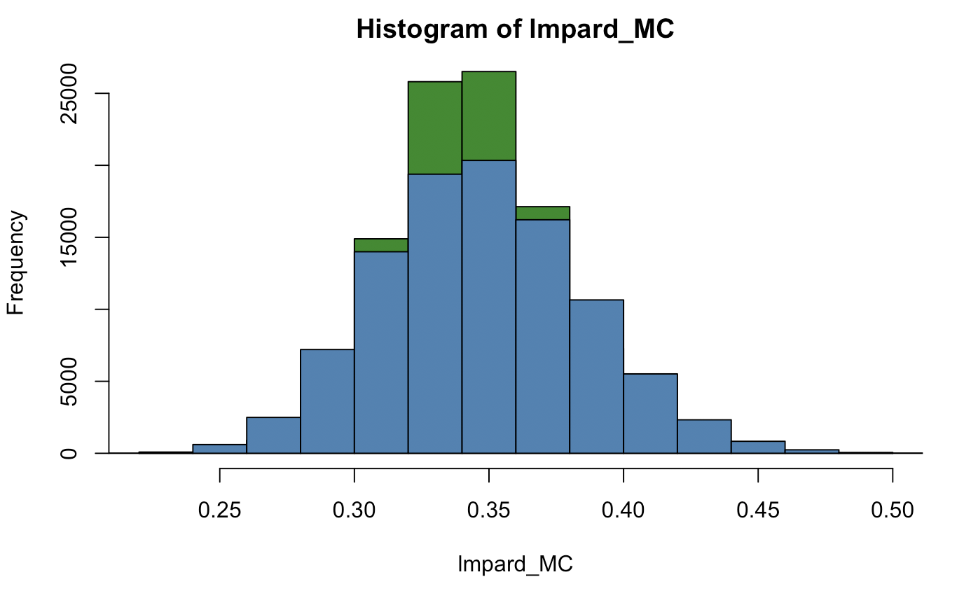
Hazard’s distribution looks wider than Lampards, but they are neatly bound. We notice that having more data definitely does help. Now let’s make the comparison, is the rising star doing better (in terms of goals) than the old dog?
mean(hazard_MC-lmpard_MC>0)
## [1] 0.5293
Looking at the distributions already gives us a hint, but we see that they are quite similar to each other in terms of goals scored. A two tailed test to see if there is an absolute difference says, not really!
quantile(hazard_MC - lmpard_MC,c(.025,.975))
##        2.5%       97.5%
## -0.08721805  0.09948989
Predictions
Now let’s make some predictions. In a previous post on beta-binomial, we did similar with iphone returns; it is just the same process. The marginal likelihood including data will give us a good posterior prediction for what is to come.
For Lampard, let’s see how many goals he may have scored if he was to play another typical season with Chelsea. After some hefty computation (and the math checks out), this comes out to be a negative binomial distribution with the poisson parameter as a random variable.
# posterior predictive Lampard
theta <- rgamma(median(l_apps)*1000,la+sum(l_gols),lb+sum(l_apps))
ynew <- rpois(median(l_apps)*1000,theta)

game_sim <- colSums(matrix(ynew, nrow=median(l_apps)))
hist(game_sim) ; abline(v = median(game_sim), col = "red")
quantile(game_sim,c(.025,.5,.975))
## 2.5%   50% 97.5%
##    6    12    20

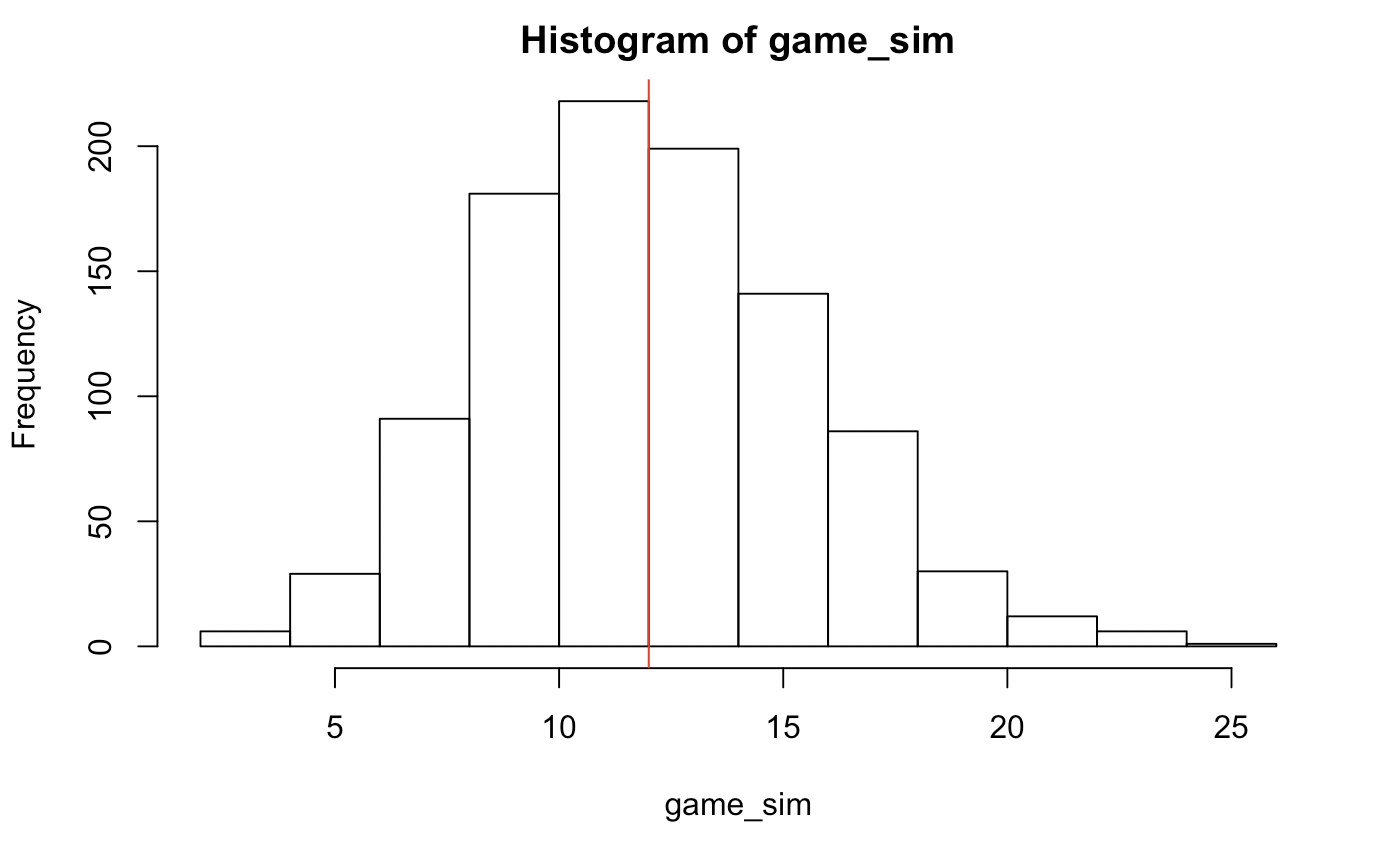
He would most likely make around 12 goals (approximate median) give or take 7. That’s quite a spread, but better than nothing! Let’s take a look at how Hazard may do finishing off this season if he were to finish off his season given that he plays a typical season.
# posterior predictive Hazard

games_left <- median(h_apps) - h_apps[length(h_apps)]
theta <- rgamma(games_left*1000,ha+sum(h_gols),hb+sum(h_apps))
ynew <- rpois(games_left*1000,theta)

game_sim <- colSums(matrix(ynew, nrow=games_left))
hist(game_sim) ; abline(v = mean(game_sim), col = "red")
qs <- quantile(game_sim,c(.025,.975))
c("lower" = qs[1], "mean" = mean(game_sim), "upper" = qs[2])
## lower.2.5%        mean upper.97.5%
##      0.000       3.129       7.000

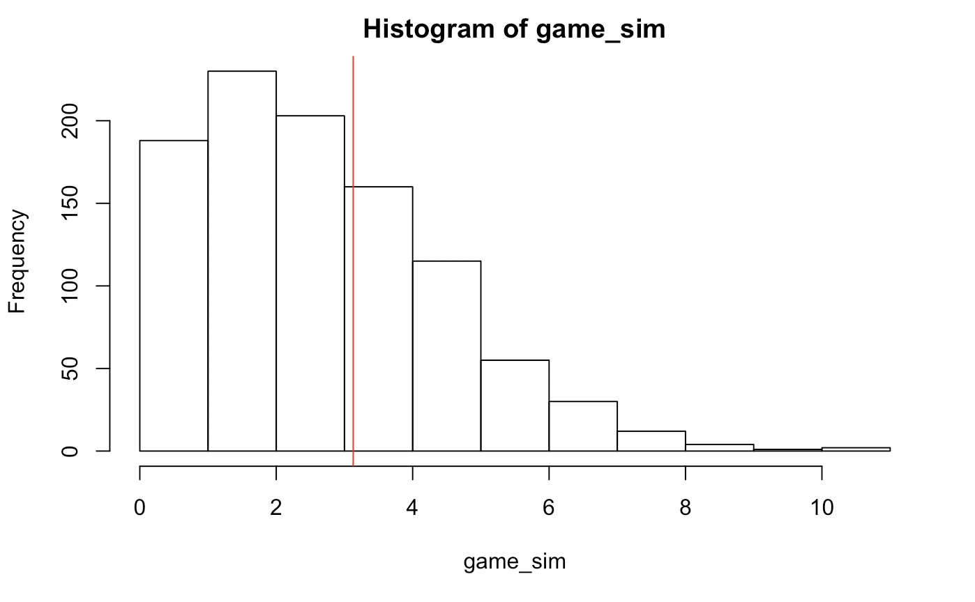
In Hazard’s last 9 games, we can expect a posterior prediction of 3 goals. Of course, we are not taking into account any cup games for chelsea nor his national or friendly appearances.
Now, granted we are making some wild predictions here. We are essentially claiming that his goal scoring is independent from each game and that he is “technically” not improving each time (a pretty Hume way to view the world). We are also not considering any other parameters such as assists, fouls, posession, etc. We are only making a “betterment” comparison using goals. Maybe to really show how great he is, comparing stats lik his assists and dribble success % may be necessary.
However, if we were blocking our factors by game we can clearly see that there is a correlation and that making a prediction is appropriate for this situation. Surprisingly, we will be very close. Isn’t this the fun of sports statistics though? We like to predict how well a player would perform but marvel when they beat the odds.