Housing and Markov Chain Monte Carlo

Case: Compring Housing Value of the top 5 wealthiest states using MCMC (may need some bayesian inference experience)

This analysis was created and curated in May of 2019.

According to U.S. News, the top 10 wealthiest states in May 2019 are as follows:

Maryland
Alaska
New Jersey
Massachusetts
Hawaii
Connecticut
New Hampshire
Virginia
California
Washington

Now, we may be safe to assume that the wealthiest states most likely have some of the highest home values in the US. Of course, we do not know this for certain, however it is a good starting point.

What model should we use?

Regular reporting may be good, however, what if you wanted to make predictions and inference on direct differences? Would regular reporting allow for this? Not really. There are various techniques, however we will be looking at the Markov-Chain Monte Carlo Method to analyze our data.

The MC MC is a bayesian method of hiearchical analysis that allows for complex integration to be done computationally. For this specific example, we will be assuming a normally distributed dataset and normally distributed prior distribution with unknown µ and σ². It is essentially doing a multi-sample t-test of differences in a Bayesian way.

It first creates two full conditional distributions for µ and σ² using gibbs sampling. These two distributions are then included as possible samples of µ and σ² to create posterior and posterior predictive distributions.

Now that (above) was a very general explanation of how the model works. However, if you are curious on the specifics, make sure to check this resource out. A general knowledge of Bayesian techniques and distributional knowledge may be necessary to complete this task. However, If for any reason you don’t really care about the statistics and you want to just do the modelling, just scroll down for the code

Wait, but are housing prices normally distributed?

Well, in all honesty, it depends. Housing prices are commonly non-normal distributions because of the way our economy is. There are fewer uber-rich people as there are lower-income. However, if transformed, this data might be taken as normally distributed.

Data

In comparing these states, we will use the Zillow dataset to look at their home value index. We are mostly interested in the Zhvi data for each state. This is data collected on homes that were displayed on their website for sale. We assume that the data is independently collected from observation to observation.

The invgamma will be necessary when including the full-conditional distribution for σ² (which we will cover in a bit).

# Packages
library(tidyverse)
library(invgamma)
library(MASS)
# Read me in!
path <- "https://raw.githubusercontent.com/tykiww/projectpage/master/datasets/housingvalue/Metro_Zhvi_Summary_AllHomes.csv"
zill <- read_csv(path)
glimpse(zill)

## Observations: 783
## Variables: 16
## $ RegionID           <int> 102001, 394913, 753899, 394463, 394514, 394974, 394692, 395209, 394856, 394347…
## $ Date               <date> 2019-02-28, 2019-02-28, 2019-02-28, 2019-02-28, 2019-02-28, 2019-02-28, 2019-…
## $ RegionName         <chr> "United States", "New York, NY", "Los Angeles-Long Beach-Anaheim, CA", "Chicag…
## $ State              <chr> NA, "NY", "CA", "IL", "TX", "PA", "TX", "DC", "FL", "GA", "MA", "CA", "MI", "C…
## $ SizeRank           <int> 0, 1, 2, 3, 4, 5, 6, 7, 8, 9, 10, 11, 12, 13, 14, 15, 16, 17, 18, 19, 20, 21, …
## $ Zhvi               <int> 226300, 440400, 652200, 225300, 244400, 233500, 206300, 406800, 284700, 218600…
## $ MoM                <dbl> 0.0031028369, 0.0034176350, -0.0007660487, 0.0022241993, 0.0057613169, 0.00300…
## $ QoQ                <dbl> 0.014343344, 0.010555301, 0.001228124, 0.010313901, 0.025167785, 0.009948097, …
## $ YoY                <dbl> 0.07200379, 0.04707561, 0.02466614, 0.03491043, 0.09990999, 0.03501773, 0.0628…
## $ `5Year`            <dbl> 0.06522199, 0.04517718, 0.06177574, 0.05122774, 0.10537396, 0.03851077, 0.0741…
## $ `10Year`           <dbl> 0.027220895, 0.012722285, 0.040997305, 0.003806871, 0.053739509, 0.006431629, …
## $ PeakMonth          <chr> "2019-02", "2006-07", "2019-01", "2007-02", "2019-02", "2007-05", "2019-02", "…
## $ PeakQuarter        <chr> "2019-Q1", "2006-Q3", "2019-Q1", "2007-Q1", "2019-Q1", "2007-Q2", "2019-Q1", "…
## $ PeakZHVI           <int> 226300, 452800, 652700, 254100, 244400, 237300, 206300, 435400, 311600, 218600…
## $ PctFallFromPeak    <dbl> 0.0000000000, -0.0273851590, -0.0007660487, -0.1133412043, 0.0000000000, -0.01…
## $ LastTimeAtCurrZHVI <chr> "2019-02", "2006-01", "2018-12", "2004-12", "2019-02", "2006-05", "2019-02", "…

Data will be first separated into just the top 10 states.

state_codes <- c('MD', 'AK', 'NJ', 'MA', 'HI')
hvi <- zill[zill$State %in% state_codes,c(4,6)] # pull only state and house value.
unique(hvi$State) %in% state_codes  %>% sum # confirm if correct.
summary(hvi$Zhvi)
rm(path,zill)

## [1] 5
##    Min. 1st Qu.  Median    Mean 3rd Qu.    Max. 
##   92200  218500  278000  331560  381600  810800 

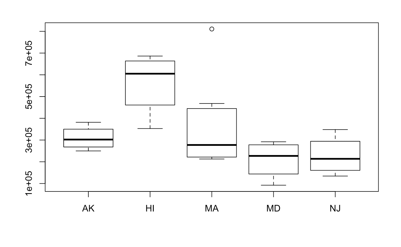
Distributions of each of the groups are as follows. Not all the data looks roughly normal, but we will have to move forward with the assumptions. Interestingly, transformations will be hard to do. This is because the variances output by the model will be large, and re-transforming the data will may make the data converge to infinity.

boxplot(Zhvi ~ State, data = hvi) 

Prior Elicitation

Now it is time to choose our prior parameters. Especially because our data is sparse, we are not so certain what the average value of homes in the top 5 states are. Accordingly, we will have to do with choosing the similar prior distributions for µ and uncertain priors for σ².

Some general ways we may choose priors::

Ask an expert what they believe to be the mean and standard deviation.
Use a time-series analysis for data per state, pick a reasonable point estimate
Do a regression analysis on income and housing prices. Predict a typical value of income for home.
Assume ignorance

Since we are working with both unknown population variance means, we will have to generate each of them. If life and math was easier, we wouldn’t lose conjugacy when assuming both unknown values. We know this cannot happen because the variance is hiearchically defined in terms of the mean.

Explanation for Priors

To find our priors, we need to first determine which models we are going to use.

µ will be distributed as a Normal with parameters m, v.
σ² will be distributed as an Inverse Gamma with parameters a, b.

Why this is so, may be found here in section 2.

Choosing our Priors

For this example, we will choose the following prior distributions (these were not all generated empirically).

X	Hawaii	Alaska	Massachusetts	Maryland	New Jersey
m	500000	278000	278000	278000	278000
v	4000	4000	4000	4000	4000
a	.01	.01	.01	.01	.01
b	.01	.01	.01	.01	.01

Here is a justification for why I chose these priors.

m
This is generally the median of the top 5 data.
Hawaii adjusted based on relative median.
v
- We want to choose a larger variance due to uncertainty.
- Real values should most likely be picked generally larger due to uncertainty.
- Depending on how much larger the spread for each state was, the variance was adjusted slightly.
a = .01
- Assuming ignorance
b = .01
- assuming ignorance

Building the Markov-Chain Model

Now here is the most interesting part. Generally, there are three steps required to create our Markov Chain model:

Create intial values for µ and σ². - We will need to initialize a vector with some starting simulated values. - These can be either µ = 0 and σ² = 1 or the mean and variance our data. - For the sake of learning, we will start with 0 and 1.

mu <- c(0) # or mu <- mean(data)
sig2 <- c(1) # or sig2 <- var(data)
# n <- length(data)
# m <- refer to chart above ; a <- refer to chart above
# v <- refer to chart above ; b <- refer to chart above
rm(mu,sig2) # we won't be using these

For i in J iterations…

a1) take a sample from full conditional (~same as posterior m*) for µ where σ<sup>2</sup>  = j-1
b1) take a sample from full conditional (~same as posterior v*) for σ<sup>2</sup> where v = j-1
c1) These full conditional values will be used to create µ<sub>j</sub>

vstar <- v * sig2[j-1] / (n * v + sig2[j - 1]) # this is the posterior v*
mstar <- (n * v * ybar + m * sig2[j - 1])/(n * v + sig2[j - 1]) # this is the posterior m*
mu[j] <- rnorm(1, mstar, sqrt(vstar)) # Generate 1 sample from full-conditional(posterior) distribution

cont… using the new mu[j] generated!! (this is one of the components that make it hiearchical)

a2) generate a full conditional (~same as posterior a*) using prior a and length n of data.
b2) generate a full conditional (~same as posterior b*) for priors b, data, and using µ<sub>j</sub>
c2) these full conditional values will be used to create σ<sup>2</sup><sub>j</sub>

astar <- a + (n/2)
bstar <- b + sum((data-mu[j])^2)/2
sig2[j] <- rinvgamma(1,astar,bstar)

The new µ_j and σ²_j values are the posterior distributions!
Predictive distributions may be chosen by generating random samples of from either the posterior or prior.

list("post-pred" = rnorm(J,mu,sqrt(sig2)), "Prior-pred" = rnorm(J,rnorm(J,m,sqrt(v)), sqrt(rinvgamma(J,a,b))))

Burn and thin samples that have not converged yet.

- Values generated by MC samples take time to converge, we will need to remove all values prior to that.
- Because each hiearchical value depends on each other, data may become heavily correlated. We may thin the data by choosing every multiple of uncorrelated data (using acf plots)

Let’s put it all together in a function!

norm_mcmc <- function(J, m, v, a, b, y) {
  #'  m, v, a, b : full-conditional priors for NN and IG
  #'  J : Monte-Carlo iterations
  #'  y : Data
  
  # Set starting values for mu, sig2
  mu <- c(0) ; sig2 <- c(1)
  # Get important values
  n <- length(y) ; ybar <- mean(y)
  
  for (j in 2:J) {
    # Create posterior for unknown mu using full conditionals
    mstar <- ((n * v * ybar) + (m * sig2[j-1])) / (n * v + sig2[j-1])
    vstar <- (v * sig2[j-1]) / (n * v + sig2[j-1])
    mu[j] <- rnorm(1,mstar,sqrt(vstar))
    # Create posterior for unknown sig^2 using full conditionals
    astar <- a + (n/2)
    bstar <- b + sum((y-mu[j])^2)/2
    sig2[j] <- rinvgamma(1,astar,bstar)
  }
  list("Posterior mu" = mu,"Posterior sig2" = sig2, "post-pred" = rnorm(J,mu,sqrt(sig2)), 
       "Prior-pred" = rnorm(J,rnorm(J,m,sqrt(v)), sqrt(rinvgamma(J,a,b))))
  # taking a looooooop of each mu and sig2, so okay to perish at certain values.
}

For practice, let’s pull out data from just Maryland and generate our posterior distribution. For J, a large value such as 100000 will suffice! Procedurally, some do 102000 to burn the first 2000 automatically. Don’t worry if NAs are produced. This is usually due to generating impossible prior predictive values. We’ll probably never need to use that distribution anyways.

mc_val <- norm_mcmc(100000, 278000, 4000, .01,.01, subset(hvi,hvi$State=='MD')$Zhvi)
lapply(mc_val, head)

## $`Posterior mu`
## [1]      0.0 210002.7 277971.8 278108.0 278063.4 278109.4
## 
## $`Posterior sig2`
## [1]           1  5610195569  8269114600 12194980759  8169307515  9448542737
## 
## $`post-pred`
## [1] -1.508377e-01  1.689168e+05  4.097918e+05  2.592844e+05  2.113386e+05  3.918210e+05
## 
## $`Prior-pred`
## [1] -1.993960e+23  8.483385e+04  1.763289e+55 -1.400694e+20 -1.579684e+34  1.044109e+13

Burning, thinning, and assessing performance

Let’s take a look at some traceplots to see how many we will need to burn.

par(mfrow = c(1,2))
plot(mc_val$`Posterior sig2`, type = 'l', col = "red")
plot(mc_val$`Posterior mu`, type = 'l', col = "blue")
par(mfrow = c(1,1))

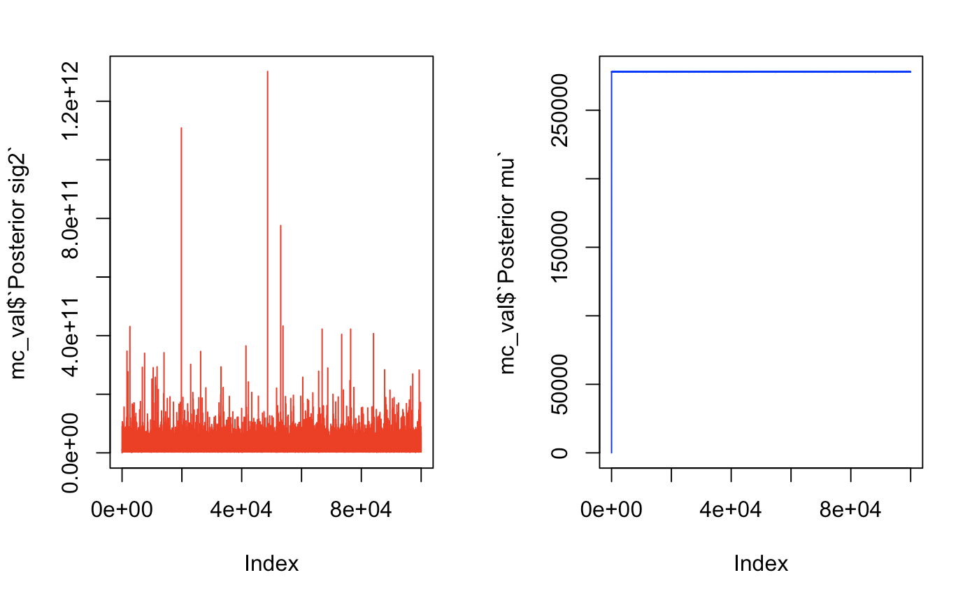
These traceplots show quick convergence. The variance looked rather healthy and converged immediately. For µ, we can take a look at the data without plotting and notice that there is a huge jump in mu from 0 to 129851 then convergence on the third value. We will burn the first 50 just to be safe. If we see a lot of oscillating, this means that we have a healthy markov chain

As for the thinning, we will observe ACF plots.

par(mfrow = c(1,2))
acf(mc_val$`Posterior sig2`)
acf(mc_val$`Posterior mu`)
par(mfrow = c(1,1))

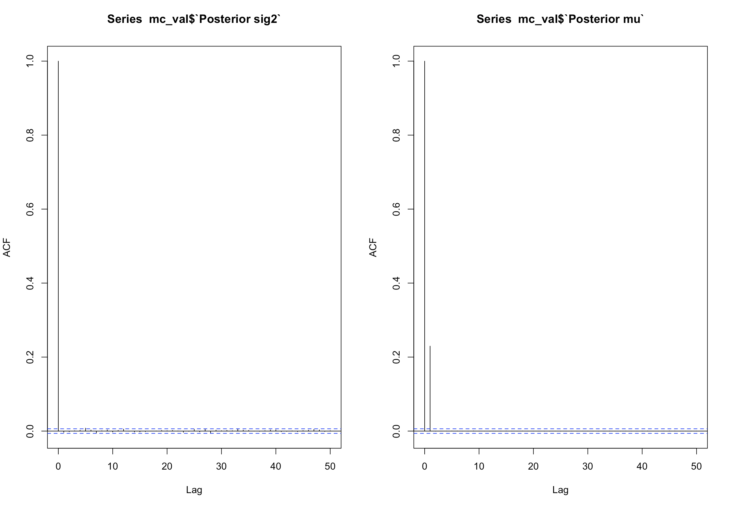
Both plots show no serious correlation in any multiple from 1-50. Usually, if there are bars that exceed the blue lines, it means there is autocorrelation. These plots are also used for time-series analysis. We will keep all our values for the Maryland posterior

# if there was autocorrelation, use something like this to grab every 10th, or 5th or whatever multiple
# seq(50:100000, by = 5)[-1] removes first 50 and takes every 5th value...
rem <- function(data,rems) data[-c(1:rems)]
mc_val <- lapply(mc_val, function(x) rem(x, 50))

Other assessments and plots can be made as follows:

2D perspective plots show that there is a relatively small variance. Using Azimuth angles, you may navigate through the latent space.

persp(kde2d(mc_val$`Posterior mu`, mc_val$`Posterior sig2`), phi = , 65,theta = 60, xlab = "µ", ylab = "sigma^2")

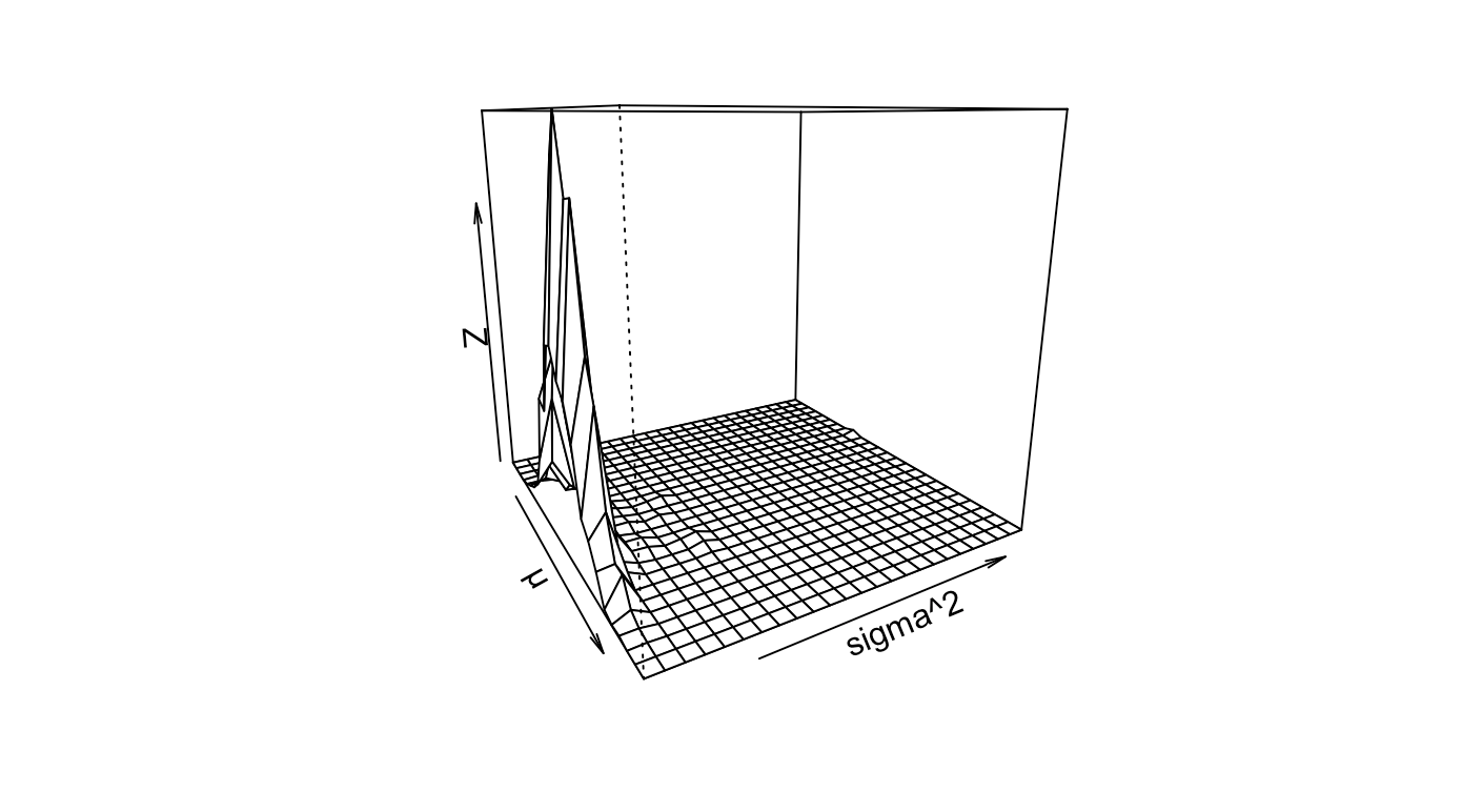
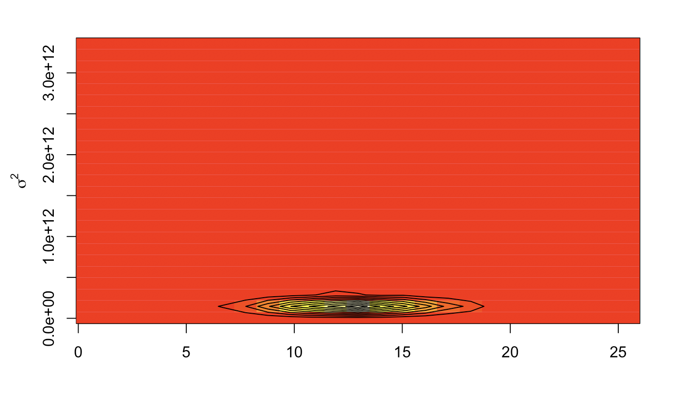
Image plots give us a heat map of the same thing from a birds eye view, a relatively precise variance. Contour lines show us the Z distribution density. This will most likely give us posterior values that are closely knit.

image(kde2d(mc_val$`Posterior mu`, mc_val$`Posterior sig2`))
contour(kde2d(mc_val$`Posterior mu`, mc_val$`Posterior sig2`), add = TRUE)
mtext(expression(sigma^2), side =2, line = 2.5)

Comparing distributions

Now here comes the real analysis. Since we have 5 different states, the proper burning and thinning will be done without explanation below (turns out, no thinning or burning is really too necessary. Our data was so small, that it immediately converged and did not affect our markov chain very much. So much for a fun analysis!).

hi_val <- norm_mcmc(100000, 500000, 4000, .01,.01, subset(hvi,hvi$State=='HI')$Zhvi)
ak_val <- norm_mcmc(100000, 278000, 4000, .01,.01, subset(hvi,hvi$State=='AK')$Zhvi)
ma_val <- norm_mcmc(100000, 278000, 4000, .01,.01, subset(hvi,hvi$State=='MA')$Zhvi)
md_val <- norm_mcmc(100000, 278000, 4000, .01,.01, subset(hvi,hvi$State=='MD')$Zhvi)
nj_val <- norm_mcmc(100000, 278000, 4000, .01,.01, subset(hvi,hvi$State=='NJ')$Zhvi)

hi_val <- lapply(hi_val, function(x) rem(x,50)) ; ak_val <- lapply(ak_val, function(x) rem(x,50))
ma_val <- lapply(ma_val, function(x) rem(x,50)) ; md_val <- lapply(md_val, function(x) rem(x,50))
nj_val <- lapply(nj_val, function(x) rem(x,50))

Distributional curves may be compared in a pariwise manner. This is the beauty of using monte-carlo sampling. Since we are looking at multiple comparisons we will start by performing a pseudo F-test (comparing the ratios of the variances). Since there are choose(5,2) = 10 possible combinations, we will only grab the most interesting looking ones.

plot(density(hi_val$`Posterior sig2`), xlim = c(0,8*10^10), ylim = c(0, 7*10^-10))
lines(density(ak_val$`Posterior sig2`), col = "blue") ; lines(density(md_val$`Posterior sig2`), col = "red")
lines(density(nj_val$`Posterior sig2`), col = "green") ; lines(density(ma_val$`Posterior sig2`), col = "brown")
legend("topright", rep(3,1), state_codes, c("red", "blue", "green", "brown", "black"))

Hawaii is not significantly larger than any of the other states because the intervals don’t contain 1. This will mean that the none of the other comparisons will yield much of a difference.

quantile(hi_val$`Posterior sig2`/md_val$`Posterior sig2`,c(.025, .975))
quantile(hi_val$`Posterior sig2`/nj_val$`Posterior sig2`,c(.025, .975))
quantile(hi_val$`Posterior sig2`/ak_val$`Posterior sig2`,c(.025, .975))
quantile(hi_val$`Posterior sig2`/ma_val$`Posterior sig2`,c(.025, .975))

##       2.5%      97.5% 
##  0.3191672 18.3357108 
##       2.5%      97.5% 
##  0.2375116 22.1070397 
##       2.5%      97.5% 
##  0.6402673 58.4333022 
##       2.5%      97.5% 
## 0.07318601 3.67102904 

We may surmise here that Hawaii is NOT significanty different from the rest of the states. HOWEVER, there is a practical significance here. Hawaiian homes on average are 222,000 dollars larger on average than Maryland homes. This is not a trivial difference.

quantile(hi_val$`Posterior mu` - md_val$`Posterior mu`,c(.025, .975))

##     2.5%    97.5% 
## 221825.5 222174.9 

Posterior probabilities may also be discovered.

mean(nj_val$`Posterior mu` < 278*10^3)

## [1] 0.4996398

The posterior probability of observing a home in New Jersey that costs less than 278k is close to 50%. These tight distributions are most likely due to having not enough data to inference off of.

Posterior Predictive

Predictive distributions were also included in the formula. These predictives have a support from (-inf,inf) so it might be normal. The distribution is larger than just the posterior.. The posterior predictive probability of the next home in Alaska being larger than 300k is below:

mean(nj_val$`post-pred`>300*10^3)

## [1] 0.4170285

Conclusion

Overall, this analysis was very simple. There are 4 key takeaways:

1) Best to have data that is as normally distributed as possible 2) The posterior distribution really made a large effect on the outcomes of our model 3) Data sufficiency is very important. Our overall posterior was very tight knit close to the data. 4) Always remember where the data comes from. This is a representative sample of zillow home sellers.

There are so many assumptions to be made while working with simulation models. However, there are so many benefits as well! Modelling heiarchical models may be applied in various settings (marketing, supply-chain, machine learning, etc). Knowing the basics definitely pays off. Go try this with a new dataset!