I’m an R guy, and when I’m asked to use other types of software, the first thing I think up of is.. How can I integrate this with R? Come Alteryx: a software company based in Irvine, California.

It’s mission is to make data science readily available and easier to use for both coders and non-coders. After using it for some time, I have come to appreciate greatly the capacity for it’s immediate vizualization, documented mapping, and strucured problem solving approach. Excel shuts down at less than 1M rows, but Alteryx can handle hundreds of millions. Alteryx compares with BI software companies such as PowerBI, SPSS, Salesforce, and Sisense. Yet, it is seen more as an “end to end” Saas product.

In my opinion, Alteryx has tried a bit too hard to be an omni machine. Probably better suited towards a non-coding audience, but there is word that more top-level companies are seeking to buy in due to excel becoming “out-dated”. I thought, I’d better start learning it.

Unfortunately, the software is only available for windows and I own a nice mac and a junk mac (got that one at a garage sale). Fortunately, we have tools such as VMware and Virtualbox to give us some help on how to get in. I won’t be explaining how to do that, I’ll just assume that you don’t have a mac and just move along! If you get stuck or need some help, take a look at this site here.

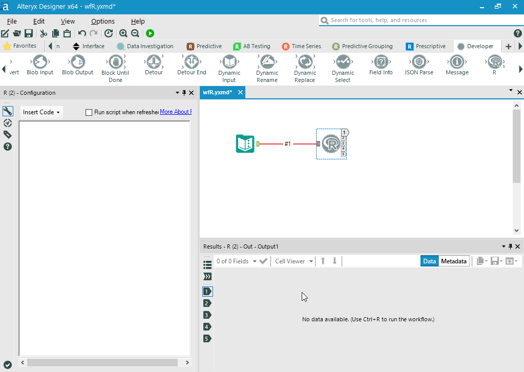
Under the assumption that you are all ready and installed, we will begin. Take a look at our basic workflow.

We’ll begin by dragging our “Text Input” node onto our workflow and put in some random numbers. I just chose to create variable a:j, 1:10, square it, then divide it by 3 (a bit mundane if you ask me, but let’s pretend that the data already existed). This is a subsitute for regular data. I would much rather show you how to work R with a smaller dataset than with one that I already work with.

Next, I’ll click on the developer pane. If you don’t have it, just press the + button on the top right, and it will let you get the options (and if you don’t even have that, you’re screwed. Just kidding. Talk to your administrator and they can sort out permissions for you). Find the R tool, and drag it onto your workflow. Alternatively, you can just type “R tool” into the search bar and it will come up for you.

Make sure it matches with the node on the text input pane. Once you see the line connected, you’re good to go. The #1 establishes the original connection and is deemed the connection “name”, so when you call it out, you just need to reference the immediate datafile, then input “#1”.

Now here comes the fun part (the R part is the fun part if you ask me). Inside our script console, we now have access to a blank R script. With it, we can basically use it to our leisure! The R module comes pre-packaged with a ton of libraries; tidyr, dplyr, ggplot2, etc.. Even the outdated zoo package is contained in there. You’re welcome to install more packages, but for the most case, you should be just fine.

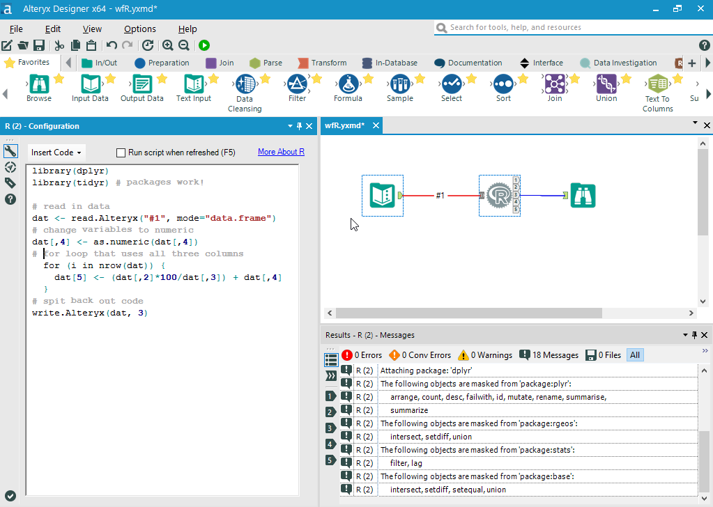
I decided to test 3 things. 1. It’s library usage 2. variable handling 3. basic coding and arithmetic capabilities. Here is my code:

library(dplyr) # packages
library(tidyr)

# Read in dataset.
dat <- read.Alteryx("#1", mode="data.frame")
dat[,4] <- as.numeric(dat[,4])
# for loop & arithmetic.
for (i in 1:nrow(dat)) {
  dat[,5] <- (dat[,2]*100/dat[,3]) + dat[,4]
}
# spit it back out.
write.Alteryx( dat , 3 )

Pretty simple stuff. Before you run the script (Ctrl + R), make sure to drag and drop the binoculars from you “favorites” tab.

Funny how it takes a bit longer for the code to run. Yet, I’m not complaining. They do a lot more work in the background than you may think.

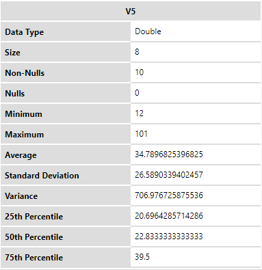
Immediately pops up the new data we calculated into a new cell. If you click on the V5 tab, it will output a summary plot statistic that looks faintly like the plotly interface (cheeky, I am very sure it is). If you hover over the plots, it will give you details on which rows and columns it is truly referring to. Manipulate it how you like, it’s very impressive.

One thing to point out, our 4th column is very wrong. If you noticed, the column should have run: 1/3, 4/3, 9/3… We notice here that the original 4/3 calculation was originally input as a string and when coerced into a float, wouldn’t budge. Makes sense, but not very convenient for us. At least we won’t be running into that problem very often if we are running data from pre-existing datasets.

A great point to note is how the summary statistics are already calculated for us. This neat tool is doing a lot of the background work for us, shaving off a lot of time.

So, it passed most of the 3 criterias. Of course, there are deeper applications to this that I have yet to show you, but it is important to note the useful nature of the integration. Now, for all you R users (and python for that matter), know that you are able to easily conquer this software with ease.