Contrary to the last post dealing with bayesian analysis, finding posterior and prior distributions are not the only things you can do with Bayesian analysis. However useful they may be, sometimes they just cannot predict future outcomes or validate your prior guesses. Here comes the prior and posterior predictive distributions.

Let’s take a marketing example. Take a look at the data below (Data below is near reported values, however returns are fictitious).
2018 Apple iPhone X vs Apple iPhone 8 Q1 Sales and Refund Table (in thousands)
| Phone | Sold Q1 | Returns Q1 | Unit Price |
|---|---|---|---|
| iPhone X | 12700 | 437 | 1.0 |
| iPhone 8 | 8500 | 277 | 0.629 |
In the realm of handheld phones, Apple is the largest giant of this day. Let’s assume (given the data) that you are looking at the performance of your two best sellers. However, as with any product, the return rates are always concerning. Refund policy is 30 days, but the data shows a surprising amount of users refunding. As a standard, you have benchmarked that a continued (3 quarters) refund rate of over 3% for 3 quarters signals a need for a re-vamp, re-call, new release, or upgrade in hardware.
Let’s explore our data and answer two questions to make some predictions on performance.
- How much better is iPhone X doing in comparison to iPhone 8? Or is it the opposite?
- What is the prior probability of return failures?
- What is the prior predictive probability of having over 30% returns on both items if they sold the same volume?
To answer number one and two, let’s use our current statistics as prior guesses.
# ipx Beta(437,12263)
a <- 437 ; b <- 12263
a1 <- 277 ; b1 <- 8223
xx <- seq(0,1,length.out = 1001)
plot(xx,dbeta(xx,a,b), type = "l", col = "maroon", xlim = c(0,.06))
# ip8 Beta(277,8223)
lines(xx,dbeta(xx,a1,b1), col = "steel blue")

# 95% credibility intervals for the proportion of returns made on each phone
c("lower" = qbeta(.025, a, b), "estimate" = a/(a + b), "upper" = qbeta(.975, a, b))
c("lower" = qbeta(.025, a1, b1), "estimate" =  a1/(a1 + b1) ,"upper" = qbeta(.975, a1, b1))
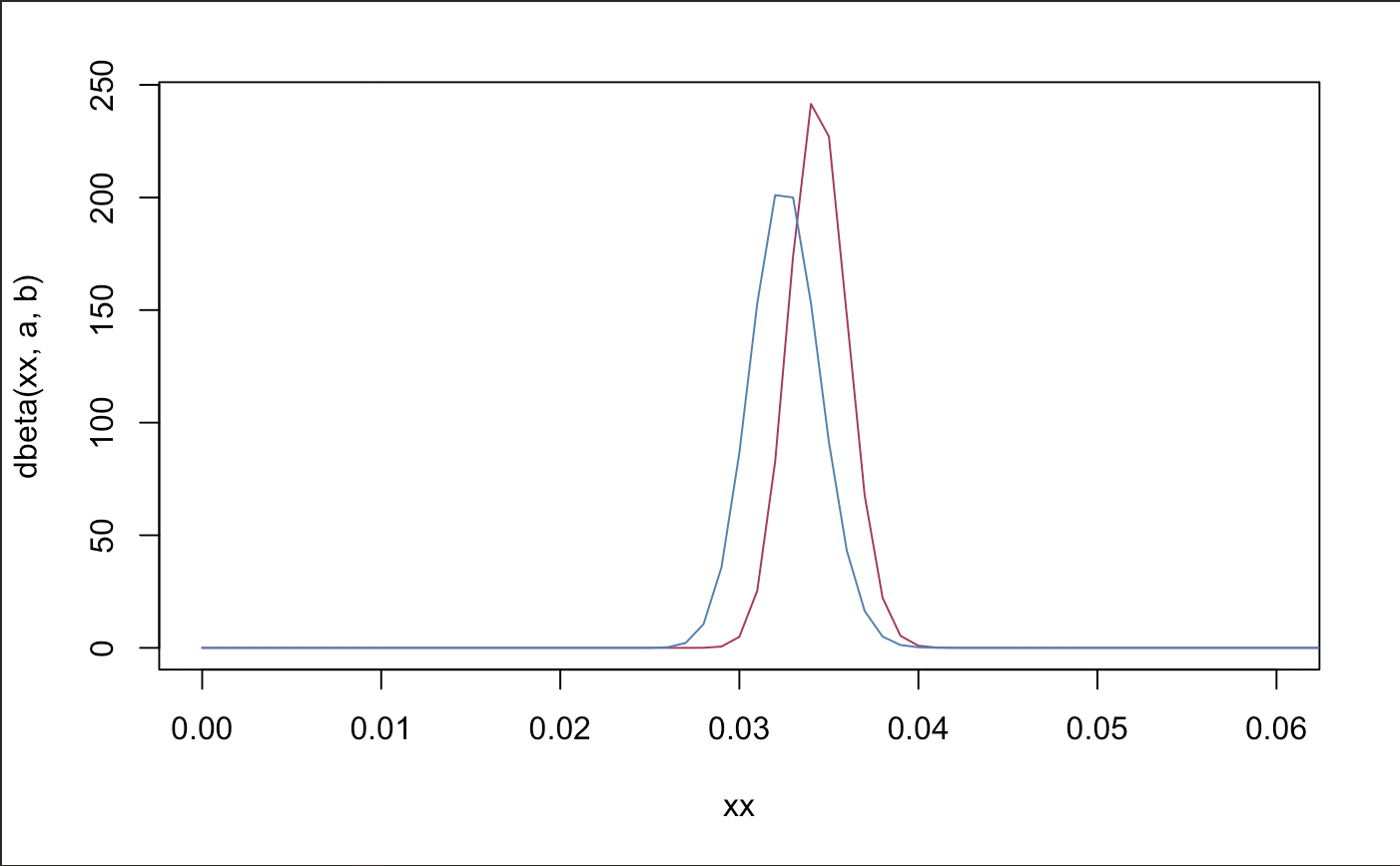
##      lower   estimate      upper
## 0.03130947 0.03440945 0.03764830
##      lower   estimate      upper
## 0.02891914 0.03258824 0.03646562
So far, we see no statistical difference in distributions, however the iPhone 8 seems to be doing slightly better in terms of refund rates. The average refund rate for the X and 8 is 3.4% and 3.2% respectively.
To answer number two:
# 3 percent returns for same data.
cutoff <- .03*12700 ; cutoff1 <- .03*8500
# Prior Predictive Distributions (has not changed because we have not observed new data)
# ipx
theta <- rbeta(100000, a,b) ; ynew <- rbinom(100000,12700,theta)
# ip8
theta1 <- rbeta(100000, a1,b1) ; ynew1 <- rbinom(100000, 8500, theta1)

mean(ynew >= cutoff) ; mean(ynew1 >= cutoff1)
## [1] 0.97682
## [1] 0.83548
This is disconcerting. Assuming the prior and that we will make similar volume in sales, we are 97% (X) and 83.7% (8) likely to get more than 3% returns.
After hearing customer feedback and making some changes and updating new features, all we do on this project is to wait until Q2 to see how we have performed.
2018 Apple iPhone X vs Apple iPhone 8 Q2 Sales and Refund Table (in thousands)
| Phone | Sold Q2 | Returns Q2 | Unit Price |
|---|---|---|---|
| iPhone X | 15660 | 441 | 1.0 |
| iPhone 8 | 18782 | 200 | 0.629 |
Now let’s make some posterior inferences from the information we have now.
- What is the new posterior probability of returns?
- With this new information, how much better is one iphone doing in comparison to the other?
- What is the new posterior predictive probability given a new sales forecast?
Again, we may answer the first questions as such (if you are at all puzzled at how this is done, take a look at this post):
# Creating posterior distribution
astar <- a + 441 ; bstar <- 15560 - 441 + b
astar1 <- a1 + 200 ; bstar1 <- 18782 - 200 + b1
nReps <- 100000
# new monte carlo distributions
theta <- rbeta(nReps, astar, bstar)
theta1 <- rbeta(nReps, astar1, bstar1)

round(mean(theta<theta1),4) # iPhone 8, whoah.
## [1] 0
Our new posterior probabilities is given by a star and b star. iPhone X now has a Beta(878,27382) distribution and the iPhone 8 has a Beta(477,26805) distribution. iPhone 8 clearly overshadowed the performance of returns compared to iPhone X. Their distributions don’t even come close.
Our cutoff performance for next quarters sales will look as follows (remember, top is X and bottom is 8):
# 95% credibility intervals for the proportion of returns made on each phone
paste("Approximate probabilities of iPhone returns.")
c("lower" = qbeta(.025, astar, bstar),"estimatae" = astar/(astar + bstar) , "upper" = qbeta(.975, astar, bstar))
c("lower" = qbeta(.025, astar1, bstar1), "estimate" = astar1/(astar1 + bstar1),"upper" = qbeta(.975, astar1, bstar1))
## [1] "Approximate probabilities of iPhone returns."
##      lower  estimatae      upper
## 0.02907744 0.03106865 0.03312272
##      lower   estimate      upper
## 0.01596261 0.01748406 0.01907249
There is most definitely a statistical difference between the two intervals. Both phones have done better in reducing returns. However, iPhone X is still on it’s way. Let’s make some predictions to see if we are on our way.
After receiving word that our sales forecast for the iPhone X will be 2% lower than previous, and the iPhone 8 will gain some traction for this next quarter by increasing 1.5%. Let’s make some cutoff values for our new forecast and see what our posterior probability of getting more than 3% returns.
# 3 percent returns for same data.
cutoff <- .03*15660*(.98) ; cutoff1 <- .03*18782*(1.015)
# Posterior Predictive Distributions
# ipx
theta <- rbeta(100000, astar,bstar) ; ynew <- rbinom(100000,round(15660*(.98)),theta)
# ip8
theta1 <- rbeta(100000, astar1,bstar1) ; ynew1 <- rbinom(100000, round(18782*(1.015)), theta1)

mean(ynew >= cutoff) ; mean(ynew1 >= cutoff1)
## [1] 0.72765
## [1] 0
Wow, we see a clear difference in performance! Based on the priors we chose and the observed data, the approximate posterior predictive probability of receiving greater than 3% returns are 72% (X) and 0% (8) given our new sales observations. Now what needs to be done is to provide a bit more improvement for the iPhone X to reduce that probability below 50%.
Hopefully this has sparked some realizations on how bayesian estimation can be used in our workforce. Especially as a KPI, bayesian techniques are fantastic in giving us approximately accurate predictions based on the information we currently have. As a business analyst, the implications of an estimation technique as such may be the key to measuring better performance. However, we must remember to be careful not to violate some assumptions or we may come out with less than attractive numbers.
Good luck on your next analytics project!