Let’s look at several methods to see if a particular event had an effect over time. This time Series Analysis seeks to analyze earned income tax credits and evaluates different models on how they can show the impact of an event.

What are Earned Income Tax Credits?
As an introduction, earned income tax credits are credits given to lower income families with children that encourages work and offsets income taxes.
“When filing taxes … working families with children that have annual incomes below about $41,100 to $56,000 (depending on marital status and the number of dependent children) may be eligible for the federal EITC. Also, working-poor people who have no children and have incomes below 15,570 (21,370 for a married couple) can receive a very small EITC. In the 2017 tax year, over 26 million working families and individuals in every state received the EITC” (source).
The EITC was enacted well in the 1970s, but has changed over time. In 1994, Policy 103-66 was enacted which increased the maximum credit for individuals with children (source). Data here looks at the efficacy of this new policy in terms of engaging more individuals to work.
library(tidyverse, verbose = FALSE)
url <- "https://raw.githubusercontent.com/tykiww/projectpage/master/datasets/EITC/income_tax_credit.csv"
dat <- read_csv(url)
dat <- dplyr::select(dat, -X1)
skimr::skim(dat) # no missing data.
## Skim summary statistics
##  n obs: 13746
##  n variables: 11
##
## -- Variable type:numeric -------------------------------------------------------
##  variable missing complete     n     mean       sd     p0     p25     p50      p75      p100     hist
##       age       0    13746 13746    35.21    10.16   20     26      34       44        54    ▇▆▅▆▅▃▃▅
##  children       0    13746 13746     1.19     1.38    0      0       1        2         9    ▇▂▁▁▁▁▁▁
##      earn       0    13746 13746 10432.48 18200.76    0      0    3332.18 14321.22 537880.61 ▇▁▁▁▁▁▁▁
##        ed       0    13746 13746     8.81     2.64    0      7      10       11        11    ▁▁▁▁▁▃▂▇
##      finc       0    13746 13746 15255.32 19444.25    0   5123.42 9636.66 18659.18 575616.82 ▇▁▁▁▁▁▁▁
##  nonwhite       0    13746 13746     0.6      0.49    0      0       1        1         1    ▅▁▁▁▁▁▁▇
##     state       0    13746 13746    54.52    27.13   11     31      56       81        95    ▆▃▃▂▆▅▁▇
##    unearn       0    13746 13746     4.82     7.12    0      0       2.97     6.86    134.06 ▇▁▁▁▁▁▁▁
##     urate       0    13746 13746     6.76     1.46    2.6    5.7     6.8      7.7      11.4  ▁▂▆▇▇▃▂▁
##      work       0    13746 13746     0.51     0.5     0      0       1        1         1    ▇▁▁▁▁▁▁▇
##      year       0    13746 13746  1993.35     1.7  1991   1992    1993     1995      1996    ▇▇▁▇▇▁▆▆
Difference in Differences Model
The Difference in Differences is a econometric model that compares a treatment’s effect over longditudinal data. Particularily useful when we have samples with selection bias, the DiD model takes into account any initial heterogeneity between the beginning and ending groups. The modelcompares the differences average outcome from the treatment group before and after the treatment, then subtracting the difference in average outcome from the control before and after.
This problem can be done in both a regression and just with the outcome data (y variable). If we were to manually calculate it with our data, it would look something like this:
\[\hat{\delta}= (\bar{y}_{T,\,A}-\bar{y}_{C,\,A})-(\bar{y}_{T,\,B}-\bar{y}_{C,\,B})\]Where $\bar{y}$ is the collected dependent data and T,C,A,B is respectively: Treatment, Control, After, and Before. We can whip this out from our data below.
# Compute the four data points needed in the DiD calculation:
cntr_befr <- mean(dat$work[dat$eitc_start ==0 & dat$kids==0])
trtm_befr <- mean(dat$work[dat$eitc_start ==0 & dat$kids==1])
cntr_aftr <- mean(dat$work[dat$eitc_start ==1 & dat$kids==0])
trtm_aftr <- mean(dat$work[dat$eitc_start ==1 & dat$kids==1])

# Compute the effect of the EITC on the employment of individuals with children:
(trtm_aftr-cntr_aftr)-(trtm_befr - cntr_aftr)
## [1] 0.04479962
Alternatively, we can estimate the $\hat{\delta}$ value with a better statistical lens by running a regression using interactions between treatments and time. By using a regression, we are able to take into account other factors that may influence the treatment effect overall.
To do this, let’s begin by creating our necessary variables. We need to specify identifiers for when EITC started, individuals with greater than 1 child, placebo treatments for those that had no EITC.
# the EITC started in 1994
dat$eitc_start <- (dat$year > 1993)*1

# EITC applies only for lower income individuals with greater than one child\
dat$kids <- (dat$children >= 1)*1

## Placebo for only pre-treatment years
before_94 <- dat[dat$year <= 1993,]

# Create a fake "post treatment" dummy
before_94$post_trt <- (before_94$year >= 1992)*1
Now that this is over, we can use these results to run our regressions. Model 1 will be an interaction between time and when EITC really started. Remember the variable did is the interaction dummies between AFTER the EITC started and TREATED individuals. Other variables can be easily tacked on as long as we keep it in this interactional format below.
did_lm <- lm(work ~ eitc_start*kids, data = dat)
summary(did_lm)$coefficients
##                     Estimate  Std. Error     t value     Pr(>|t|)
## (Intercept)      0.575459734 0.008845078  65.0598825 0.000000e+00
## eitc_start      -0.002073509 0.012931360  -0.1603474 8.726098e-01
## kids            -0.129497878 0.011676313 -11.0906478 1.839206e-28
## eitc_start:kids  0.046873132 0.017158122   2.7318335 6.306339e-03
Our beta coefficient on the did is the delta, or our DiD estimator. Pretty close to our original estimate. Testing our null hypothesis that Delta is different from zero will show that we have sufficient evidence to infer that implementing the EITC had actually increased jobs.
Furthermore, we can show the change in y from the period before treatment to after the change for both the treatment and control groups. The counterfactual indicates what would have happened if there was absolutely no treatment. We’ll have to rearrange some variables in our model first.
## Plot code from Rstudio bookdown
C <- sum(coef(did_lm)[1:4])
E <- sum(coef(did_lm)[c(1,2)])
B <- sum(coef(did_lm)[c(1,3)])
A <- coef(did_lm)[1]
D <- E+(B-A)

# PLOT
plot(1, type="n", xlab="Treatment Period", ylab="jobs", xaxt="n",
     xlim=c(-0.01, 1.01), ylim=c(0.3, .7))
segments(x0=0, y0=A, x1=1, y1=E, lty=1, col=2)#control
segments(x0=0, y0=B, x1=1, y1=C, lty=3, col=3)#treated
segments(x0=0, y0=B, x1=1, y1=D, lty=4, col=4)#counterfactual

legend("topright", legend=c("control", "treated",
    "counterfactual"), lty=c(1,3,4), col=c(2,3,4))
axis(side=1, at=c(0,1), labels=NULL)
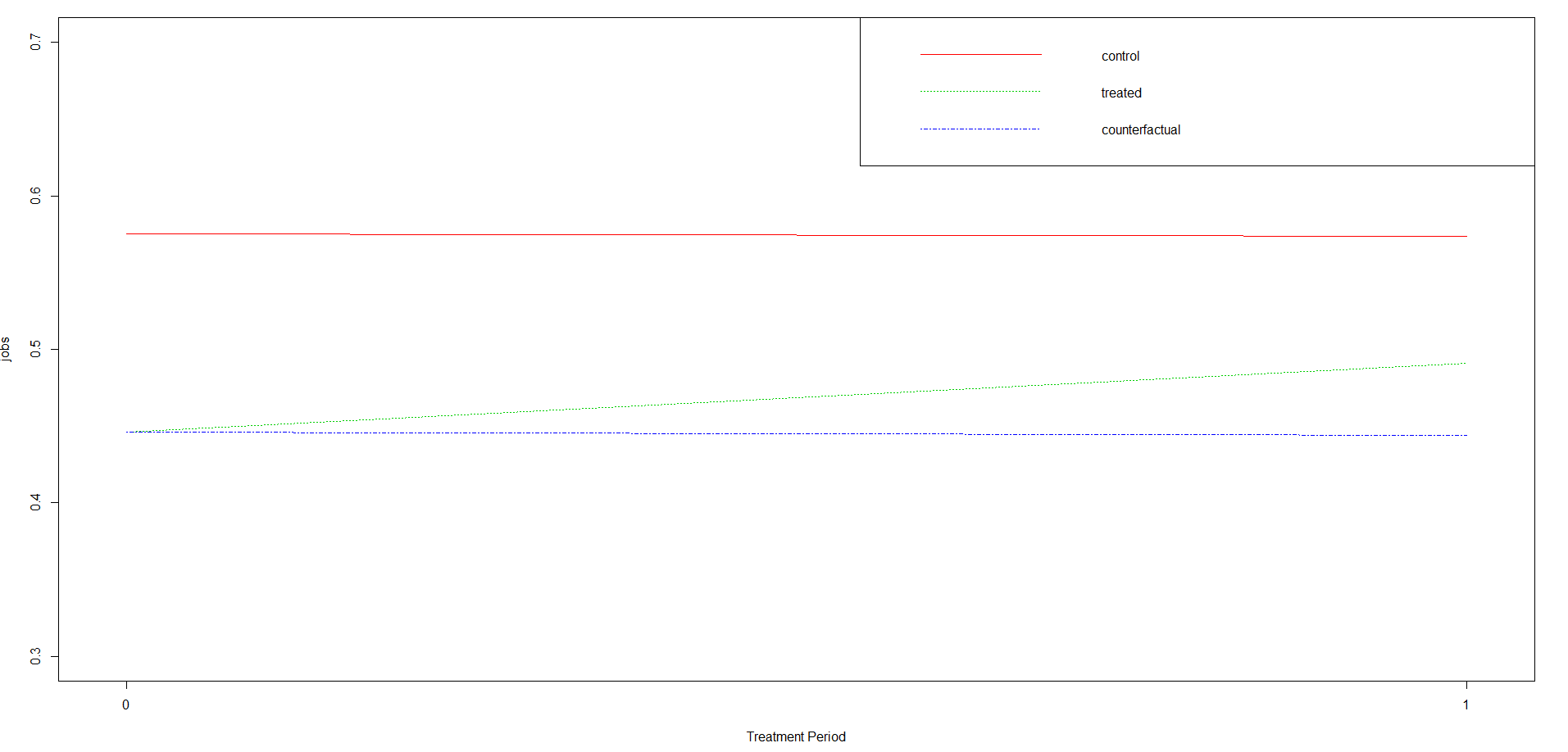
Here, we clearly see that the treatment did increase jobs overall! Our counterfactuals clearly parallel those in the control, but originating from a different intercept.
Now, if you hadn’t already realized, we broke an important assumption. Did you think it was weird that we were using a bernoulli y in an OLS regression??
The assumptions are as follows:
- The event was not determined by the outcome (no circular reference)
- Treatment and control groups have Parallel Trends in outcome
- Stable units: event and comparison is composed of stable units
- No spillover effects: Unrelated events don’t have an effect! Nothing else happened.
Technically, we have already broken one of the assumptions (2). The results are binary. Some of you may say, hey! Shouldn’t we use a logistic regression? However, it isn’t necessarily wrong to work it this way. We aren’t necessarily looking at the individual predicted values just to study if an event had an effect. Although we may have predicted values above 1 or below 0, we are just looking at the coefficients for this analysis and don’t really want to get too wrapped up in log odds transformations.
Now you know how to do a simple DiD model! We will continue to build on timeseires regresssions as we move forward.