At times, clustering can get subjective. Our goal is to use quantitative model evaluation to see if we’re doing things correct.

There are so many clustering techniques, sometimes we get confused on which ones to use. If we are to be try to be mutually exclusive about our techniques, we may separate them into 3 groups: Partitional methods, heiarchial methods, and symbolic methods.

Partitional methods produce a single partition or clustering of the data elements. Some examples include k-means, PAM, CLARA, CLARANS, etc.. Each methodology created for their uniquity in computing time, efficiency, or performance.

Heiarchial Methods produce a series of nested partitions, each of which represent a possible clustering of the data elements. heiarchial methods can work in an agglomerative (large clusters split) or divisive (small clusters grouped) way. The product is usually described in terms of dendograms. Methods include: BSP, HAC, etc.

Symbolic methods produce various algorithms. Many times the data is not in an oval cluster (heterogeneous) or we are seeking for partial clusters. In these cases we may use techniques such as: Density-based clustering and query based algorithms.

For this post, we will explore 3 different clustering methods that fit in those criterion:

• k-means
• heiarchial
• density based scanning.

Let’s begin with k-means.

library(datasets)
library(stats)
library(dbscan)
library(tidyverse)

The algorithm in code is not simple, but can be explained simply. (1) It builds k number of subsets and picks (2), randomly, an item nearest to the cluster center over and over until it converges (3). k-means does not work with categorical or factor datasets, so we are stuck with numerical values (like PAM). Furthermore, it is sensitive to outliers but does not specify any, including every point into a certain cluster. In some ways, it may be in our favor to use PAM rather than k-means. However, since PAM requires high time complexity, we will stick with our k-means algorithm.

We will use the iris dataset embedded in R (I know, very basic of me to use iris). The only line we really need to line is below.

data(iris)
# identify target cluster and computed clusters
sets <- iris[1:4] # data to cluster
tc <- iris[5] # remove target cluster

kmeans(sets,centers = k) # run algorithm for k number of clusters

However, we are looking for the optimal number of clusters, so we will explore a bit. To optimize, we will calculate their F1 scores for each value of k. If you’re curious about what an F1 score, precision, and recall are click here. Unfortunately, calculating these scores are not embedded, so we will need to create our own function. If you can think of a better way, please let me know!

# check clusters for centers 2, 3, 4, 5, 7, 9, 11
centers <- c(2, 3, 4, 5, 7, 9, 11)
iris.models <- lapply(centers, function(k) kmeans(sets,centers = k))

Below is the function for f1 score. One thing to note, is how sci-kit learn in python already has an f1 score metric (sklearn.metrics.f1_score). Maybe the best way to go about finding these scores is to run the data cleaning in tidy and send it to python. However, it is important to understand that sci-kit misses some important features crucial to statistical evaluation. We’ll just hard-code it. If anyone can find a more simple way to do this, comment below!

f1 <- function(x) {
  
  ## Function for a ##
  aa <- function(x,dataset = iris) {
    # ' Only works for iris
    # ' x stands for cluster results
    # ' dataset is predifined as iris. 
    # ' calculating a (number of pairs of items that
    # ' belong to the same cluster in both CC and TC)
    
    
    check <- 0
    for(i in 1:nrow(dataset)){
      for (j in 1:nrow(dataset)){
        if (x[i]==x[j] & dataset$Species[i]==dataset$Species[j]) {
          check <- check + 1
        }
      }
    }
    ifelse(check >=1, check <- check+1, check)
  }
  
  
  
  
  ## Function for b ##
  bb <- function(x,dataset = iris) {
    # ' Only works for iris
    # ' x stands for cluster results
    # ' dataset is predifined as iris. 
    # ' calculating b (number of pairs of items that  
    # ' belong to different clusters in both CC and TC)
    
    check <- 0
    for(i in 1:nrow(dataset)){
      for (j in 1:nrow(dataset)){
        if (x[i]!=x[j] & dataset$Species[i]!=dataset$Species[j]){
          check <- check + 1
        }
      }
    }
    ifelse(check >=1, check <- check - 1, check)
  }
  ## Function for c ##
  cc <- function(x,dataset = iris) {
    check <- 0
    for(i in 1:nrow(dataset)){
      for (j in 1:nrow(dataset)){
        if (x[i]==x[j] & dataset$Species[i] != dataset$Species[j]){
          check <- check + 1
        }
      }
    }
    ifelse(check >=1, check <- check - 1, check)
  }
  ## Function for d ##
  dd <- function(x,dataset = iris) {
    check <- 0
    for(i in 1:nrow(dataset)){
      for (j in 1:nrow(dataset)){
        if (x[i]!=x[j] & dataset$Species[i]==dataset$Species[j]) {
          check <-check + 1
        }
      }
    }
    ifelse(check >=1, check <- check - 1, check)
  }
  ## precision calculation ##
  prec <- function(x) {
    aa(x) / (aa(x)+cc(x))
  }
  ##   recall calculation  ##
  rec <- function(x) {
    aa(x) / (aa(x) + dd(x))
  }
  ## f-measure calculation ##
  precision <- prec(x)
  recall <- rec(x)
  fmeasure <- (2 * precision * recall) / (precision + recall)
  
  # c(fmeasure,recall,precision)
  
  c("f-measure" = fmeasure, "recall" = recall, "precision" = precision)
}

Our optimum is shown below given our cluster results.

# clean clusters as vectors
cluster.result <- lapply(1:length(centers), function(x) as.vector(iris.models[[x]]$cluster))

lapply(cluster.result, function(x) f1(x)[1]) %>% 
  unlist -> fmez # display f-measures

names(fmez) <- centers

which.max(fmez) # 3 clusters is the optimal K
hullplot(sets, iris.models[[2]], main = "k-means") # graphical representation of 3-means.


# library('factoextra') forprettier graphs
# fviz_cluster(iris.models[[2]], data=sets,geom='point')

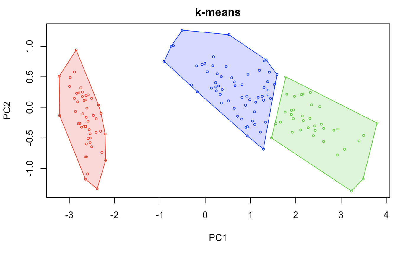
I’m not going to show how close we were to the original dataset, however this method probably fits the best out of the 3 other algorithms.

Let’s move on to heiarchial clustering.

In simple terms, heiarchial clustering assigns a data item to it’s own cluster, computes pairwise distances (min, maxm group average, centroids, etc.), merges the clusters, and repeats pairwise distances until there is no more than 1 cluster (creates a tree). The technique we will use is a “complete link” which is a maximum distance between two cluster items. This is justified because we already know that the clusters are already in globular form and not in overly large clusters. For this, an f1-score is not too necessary.

d <- dist(sets) # dist for distance matrix.
fit <- hclust(d, method="complete") # By default, the complete linkage method is used. 

plot(fit)
rect.hclust(fit,k=3) # we see 3 or 4 clusters in this dendogram
clusterCut <- cutree(fit, 3)

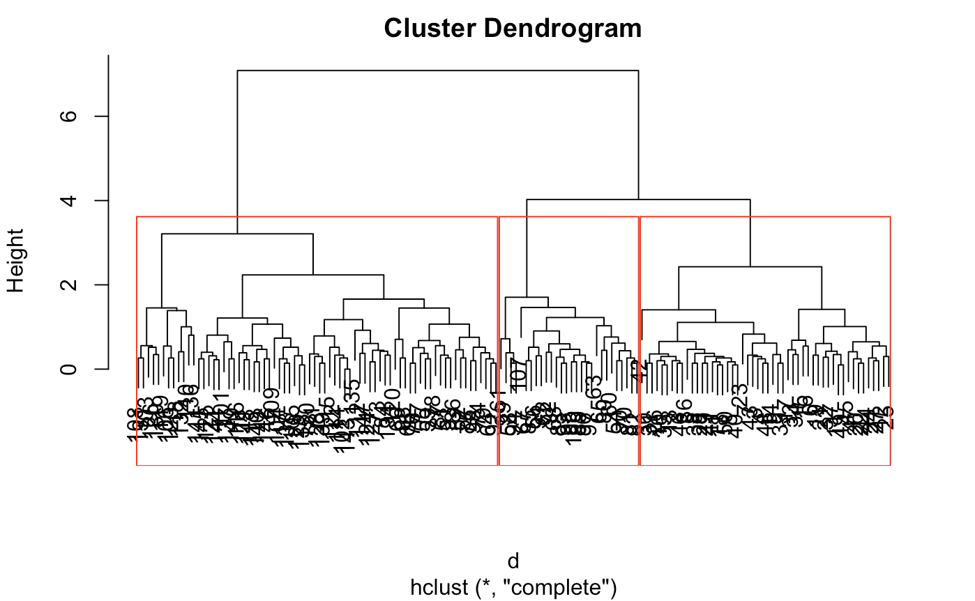
Looking at the display, The optimal threshold will be around 3 or 4 clusters. This is because the clusters are tightly bound until the number of clusters get to 4. However, because there is a slight jump from 3 to 4, we can reasonably conclude 3. In principle, we would do this by computing some quality measure, but for simplicity, we can just eyeball here. This case is not too difficult.

If you want to see a vizual representation of how close our clusters are, here is a quick ggplot.

ggplot(iris, aes(Petal.Length, Petal.Width, color = iris$Species)) + 
  geom_point(alpha = 0.4, size = 3.5) + geom_point(col = clusterCut) + 
  scale_color_manual(values = c('black', 'red', 'green'))

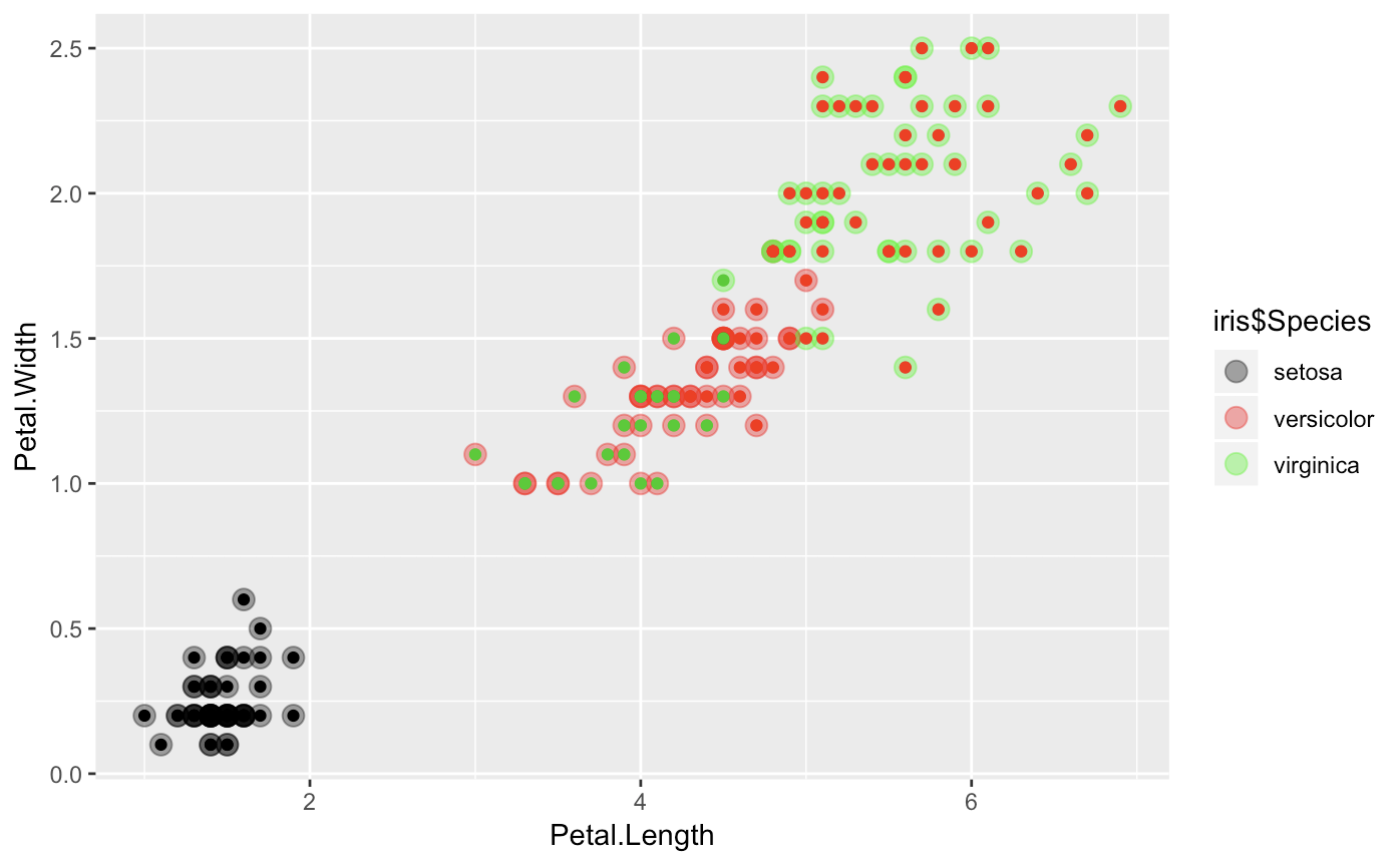
It looks a bit more mixed with some heiarchial divides (mostly in virginica and versicolor), which suggest some close relationships.

Now to our density based clustering.

This modeling technique works with non-globular data. It technically crawls and attracts points within a specified radius (density = epsilon). Core points are identified by more dense clusters (more points than minpoints). Border points are identified by groups that do not have as many points as the density, but is in the neighborhood of a core point. It seeks to eliminate “noise points” or outliers of sorts that are neither border or core points. DBscan is probably the most exotic as it is resistant to noise and can handle different shapes and sizes. However, it does have its tradeoffs. Varying densities and high-dimensional data can deter the performance of the algorithm.

iris.mat <- as.matrix(sets) # sets as matrix


epsilons <- seq(1,5,.5) # run different epsilons, 1 to 5. epsilon values take > 0 to inf.

dbscans <- lapply(epsilons,function(x) dbscan(iris.mat,eps = x)) # lapply for optimization.

# grab all f-measures
lapply(1:length(epsilons),function(x) f1(dbscans[[x]]$cluster)[1]) %>%
  unlist -> db.fmez # this line of code will take forever. Decrease epsilon values for simplicity.

which.max(db.fmez) # maximum F score given by epsilon of 1 to 1.6

factoextra::fviz_cluster(dbscans[[2]], data=sets,geom='point')

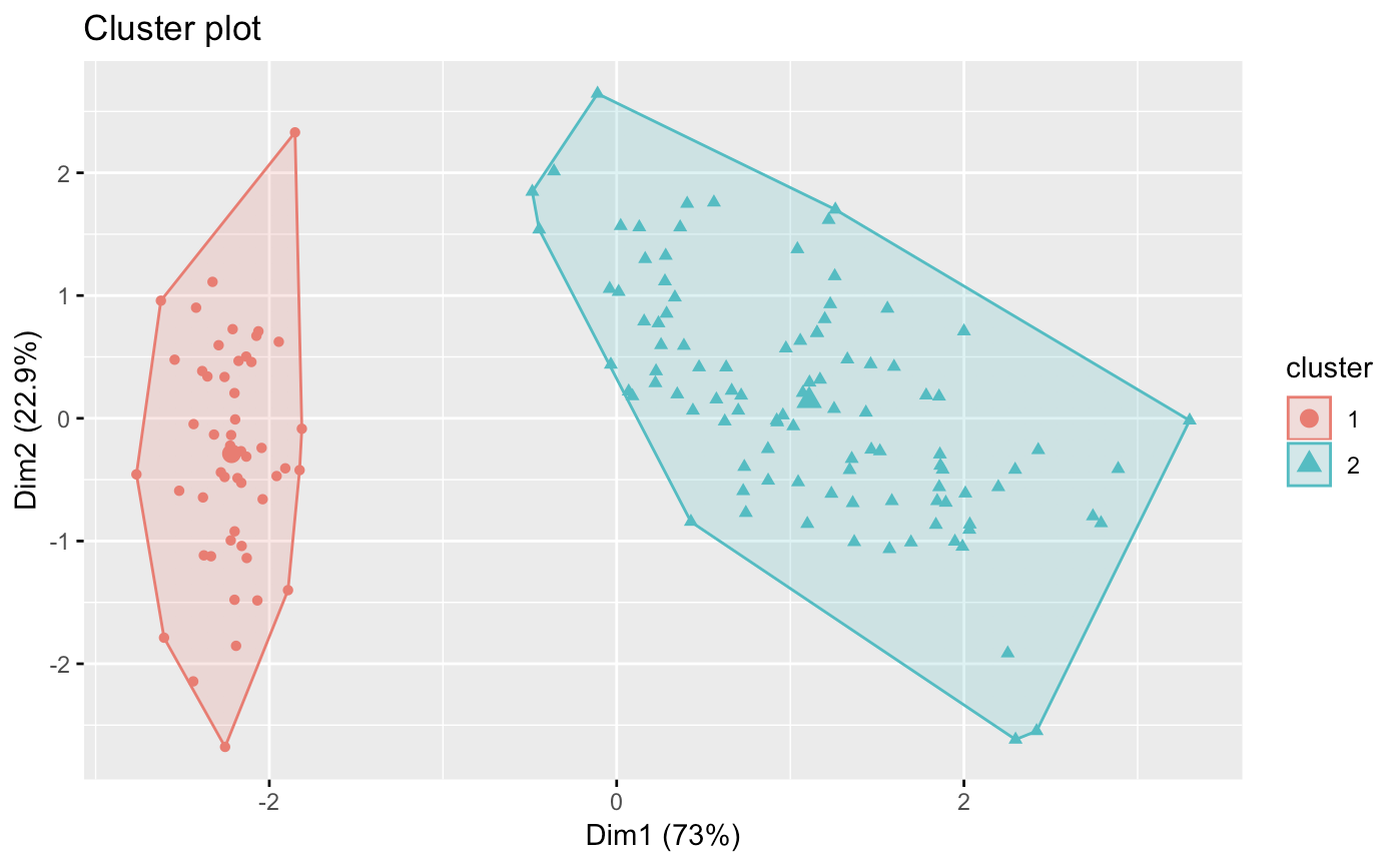
Here, we notice the downfall of dbscan for simple clustering. We notice that our accuracy decreases with values past 1.6 However, even with epsilon of 1, we only get 2 clusters.

Using these methods is an art. Many think that clustering is just something that can be done easily and is simple. However, we must understand that this is still a new field and parameters are constantly changing. Even looking at these various clusters, we notice how different each of the cluster composition and sizes are.

## cluster size and composition comparison between dbscan, hclust, and kmeans

# kmeans clusters
iris.models[[2]]$cluster %>% as.vector %>%
  factor -> kmeans

# heiarchial clusters
cutree(fit,k=3) %>% as.vector %>%
  factor -> hclusts

# dbscan clusters
dbscans[[7]]$cluster %>% as.vector %>%
  factor -> dbscanss

sapply(1:3, function(x) sum(kmeans==x)) # size of k-means cluster # 1, 2, 3
sapply(1:3, function(x) sum(hclusts==x)) # size of hcluster # 1, 2, 3
sapply(1:2, function(x) sum(dbscanss==x)) # size of dbscan cluster 1, 2


lapply(1:3, function(x) which(kmeans==x)) # Datapoints of each kmeans cluster 1,2,3
lapply(1:3, function(x) which(hclusts==x)) # Datapoints of each hcluster 1,2,3
lapply(1:2, function(x) which(dbscanss==x)) # Datapoints of each dbscan cluster 1,22
# you'll have to run the last 3 lines on your own. It shows discriminant data points.

## Sizes
## [1] 50  38  62 
## [1] 50  72  28
## [1] 50  100 

With unsupervised learning, we have to be very careful in our approach with data. It’s more of an art than anything else. Sometimes clustering takes a bit to get used to, however, it will be a useful tool for any type of segmentation analysis!