This is a continuation (a part II) from the Cox Proportional Hazards regression. Even if you don’t read the last post, it is okay. We won’t be covering much of the CPH model. Let’s get started with our survival model.
Brief Summary: AFT regression.
- Uses a time and right censor (0 or 1) data to predict the survival probability given covariates.
- Data we have has
tenureandChurnwhich is what we use to model survival. tenure is how longa customer has been with the company. churn is whether or not a customer has left (or perceived to have left) - Model fitting is really easy. The model does better when you dummy/one-hot/assume fixed effects.
- Assumes covariate acts multiplicatively on time. p-value for coefficient should NOT be significant for a well fitted covariate.
- hypothesis asks if the covariate is proportional to distribution quantile or not. If NOT proportional, p-value is significant. We need some sort of proportionality.
The problem we had earlier was… We have a duration model that did not meet its assumptions. Although the Cox Proportional Hazards model was a censored regression that included a time weighting, our proportionality assumptions did not meet.
What if we can sidestep the linear time proportionality assumption and only worry about censorship, residuals, and independence? What would we have to do? We would then have to think of something that is more parametric to meet any immediate assumptions. In fact, there is! An Accelerated Failure time Model.
Instead of covariates acting multiplicatively on the hazard, we can assume that covariates act multiplicatively on time. In other words, instead of a unit change in a covariate reduces/increases a hazard by a certain (x) factor, we can say that a unit change in in a factor shortens/increases survival time by x times. By doing so, we can introduce a distribution for a more parametric approach.
Furthermore, we do NOT need to worry about linear proportionality with time. We now should be worried about time-quantile proportionality. In simpler terms, our null hypothesis is that the time and the quantile (x axis of the distribution) are proportional to each other, still close to 1. As long as we have the right distribution, our p-values shouldn’t be significant at all!
The code is a lot simpler than the CPH model. Description on the data was provided in the last entry.
library(tidyverse, quietly = TRUE)
url <- "https://raw.githubusercontent.com/treselle-systems/customer_churn_analysis/master/WA_Fn-UseC_-Telco-Customer-Churn.csv"
data <- read_csv(url)
skimr::skim(data)
## Skim summary statistics
##  n obs: 7043
##  n variables: 21
##
## -- Variable type:character -----------------------------------------------------
##          variable missing complete    n min max empty n_unique
##             Churn       0     7043 7043   2   3     0        2
##          Contract       0     7043 7043   8  14     0        3
##        customerID       0     7043 7043  10  10     0     7043
##        Dependents       0     7043 7043   2   3     0        2
##  DeviceProtection       0     7043 7043   2  19     0        3
##            gender       0     7043 7043   4   6     0        2
##   InternetService       0     7043 7043   2  11     0        3
##     MultipleLines       0     7043 7043   2  16     0        3
##      OnlineBackup       0     7043 7043   2  19     0        3
##    OnlineSecurity       0     7043 7043   2  19     0        3
##  PaperlessBilling       0     7043 7043   2   3     0        2
##           Partner       0     7043 7043   2   3     0        2
##     PaymentMethod       0     7043 7043  12  25     0        4
##      PhoneService       0     7043 7043   2   3     0        2
##   StreamingMovies       0     7043 7043   2  19     0        3
##       StreamingTV       0     7043 7043   2  19     0        3
##       TechSupport       0     7043 7043   2  19     0        3
##
## -- Variable type:numeric -------------------------------------------------------
##        variable missing complete    n    mean      sd    p0    p25     p50     p75    p100     hist
##  MonthlyCharges       0     7043 7043   64.76   30.09 18.25  35.5    70.35   89.85  118.75 ▇▁▃▂▆▅▅▂
##   SeniorCitizen       0     7043 7043    0.16    0.37  0      0       0       0       1    ▇▁▁▁▁▁▁▂
##          tenure       0     7043 7043   32.37   24.56  0      9      29      55      72    ▇▃▃▂▂▃▃▅
##    TotalCharges      11     7032 7043 2283.3  2266.77 18.8  401.45 1397.47 3794.74 8684.8  ▇▃▂▂▁▁▁▁
Here is the same cleaning.
# binary removal
condition <- data[,apply(data,2,function(x) length(unique(x)))==2]
later <- colnames(data)[!colnames(data) %in% (condition %>% names)]
binary <- ifelse(condition=="Yes"| condition=="Female" | condition == 1,1,0)
new_data <- cbind(dplyr::select(data,later),binary) %>% as_tibble
# NA removal
new_data <- na.omit(new_data)
# Customer ID Removal
new_data <- dplyr::select(new_data,-customerID)
# Dummy the data
# fixed effects
library(fastDummies)
dummy_data <- fastDummies::dummy_cols(new_data,remove_first_dummy = TRUE)[-c(2:11)]

# split data
set.seed(15)
idx <- sample(nrow(dummy_data),3, replace = FALSE)
test_dat <- dummy_data[1:nrow(dummy_data) %in% idx,-c(1,10)]
dum_data <- dummy_data[!1:nrow(dummy_data) %in% idx,]
Now that we have the basic hygeine out of the way, let’s get started on the modelling.
library(survival)
library(survminer)
The first step is determining a possible distribution for the y variable tenure. TLet’s first plot the data.
hist(new_data$tenure,breaks = 50)
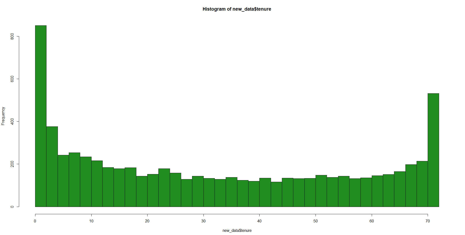
It seems to be a heavily right-tailed distribution with a possible bimodal nature. However, we have to remember that this is right-censored data so there is a possibility that we have unobserved tenure that extends longer. Understanding this, the distribution seems less scary.
Some possible candidates may be a gamma, weibull, exponential, or lognormal. The model seems to take a weibull, exponential, or lognormal unless we just create our pdf on our own. Now, we can figure this out two ways. 1, use fitdistr(), fitdist(), decdist() or any of their likeness. 2, just try them all and see which has the best log-likelihood.
Let’s just do the simpler one.
# Creating a formula and removing tenure and churn
cols <- colnames(dum_data)[!(colnames(dum_data)%in% c("tenure","Churn"))]

form <- as.formula(paste("Surv(tenure,Churn) ~ `",paste(cols, collapse='` + `'),'`', sep = ""))

# Model saved using weibull as distribution (default)

dists <- c("weibull", "exponential","lognormal")

check_likelihood <- function(x) {
  rez <- survreg(form, data =  dum_data, dist = x)
  return(rez$loglik[1])
}

# Check the fit of the models.
sapply(dists,function(x) check_likelihood(x))
##    weibull exponential   lognormal
##  -10571.24   -10842.34   -10513.64
It seems like the exponential has the lowest log-likelihood (-2 * log(lik) to be precise). This is a good thing. The Likelihood ratio test checks to see whether adding certain variables to the existing model improves the model fit or not. The existing model is the null (intercept). If the likelihood is better than the intercept, it fits better. Though not an ouput for this code, a p-value usually accompanies the LRT. If the p-value is not significant (p < 0.05) it means that adding variables to the null model is not significantly reducing the log likelihood.
Let’s try this output.
aft_model <- survreg(form, data = dum_data, dist = "exponential")
summary(aft_model)
## Call:
## survreg(formula = form, data = dum_data, dist = "exponential")
##                                               Value Std. Error     z       p
## (Intercept)                                3.03e+00   6.97e-01  4.34 1.4e-05
## MonthlyCharges                            -6.45e-04   2.29e-02 -0.03   0.978
## TotalCharges                               7.59e-04   2.31e-05 32.89 < 2e-16
## gender                                    -2.55e-02   4.64e-02 -0.55   0.583
## SeniorCitizen                             -4.35e-02   5.66e-02 -0.77   0.442
## Partner                                    1.39e-01   5.43e-02  2.55   0.011
## Dependents                                 1.36e-01   6.92e-02  1.97   0.049
## PhoneService                              -2.10e-01   5.83e-01 -0.36   0.718
## PaperlessBilling                          -1.64e-01   5.69e-02 -2.88   0.004
## MultipleLines_No                           2.45e-02   1.25e-01  0.20   0.845
## MultipleLines_Yes                          0.00e+00   0.00e+00    NA      NA
## `InternetService_Fiber optic`             -8.60e-01   5.76e-01 -1.49   0.135
## InternetService_No                         1.30e+00   7.01e-01  1.86   0.063
## OnlineSecurity_Yes                         2.75e-01   1.32e-01  2.08   0.037
## `OnlineSecurity_No internet service`       0.00e+00   0.00e+00    NA      NA
## OnlineBackup_No                           -6.34e-02   1.27e-01 -0.50   0.616
## `OnlineBackup_No internet service`         0.00e+00   0.00e+00    NA      NA
## DeviceProtection_Yes                      -1.14e-02   1.26e-01 -0.09   0.928
## `DeviceProtection_No internet service`     0.00e+00   0.00e+00    NA      NA
## TechSupport_Yes                            1.94e-01   1.32e-01  1.47   0.142
## `TechSupport_No internet service`          0.00e+00   0.00e+00    NA      NA
## StreamingTV_Yes                           -2.07e-01   2.35e-01 -0.88   0.378
## `StreamingTV_No internet service`          0.00e+00   0.00e+00    NA      NA
## StreamingMovies_Yes                       -1.97e-01   2.34e-01 -0.84   0.401
## `StreamingMovies_No internet service`      0.00e+00   0.00e+00    NA      NA
## `Contract_One year`                        7.43e-01   9.15e-02  8.11 4.9e-16
## `Contract_Two year`                        1.67e+00   1.65e-01 10.13 < 2e-16
## `PaymentMethod_Mailed check`               6.13e-03   7.10e-02  0.09   0.931
## `PaymentMethod_Bank transfer (automatic)`  3.36e-01   7.17e-02  4.68 2.8e-06
## `PaymentMethod_Credit card (automatic)`    3.95e-01   7.47e-02  5.29 1.2e-07
##
## Scale fixed at 1
##
## Exponential distribution
## Loglik(model)= -8272.3   Loglik(intercept only)= -10842.3
## 	Chisq= 5140.01 on 29 degrees of freedom, p= 0
## Number of Newton-Raphson Iterations: 7
## n= 7029
Here is also the survival curve for the model intercept for your reference
intercept <- 2.52
xx <- seq(0,70,length.out = 1001)
# survival probability of intercept. As time increases, overall survival decreases as such.
plot(xx,1-pexp(xx,exp(-intercept)),xlab="t",ylab=expression(hat(S)*"(t)"))
This just shows that if nothing were to occur, this is the survival probability of a given customer over time. After t ~ 8,
Let’s get back to the coefficients table.
Now the interpretation here is a bit different. The p-values on the right indicate whether or not a particular covariate is proportional or not to survival distribution. We assume that the log of the survival times is affected linearly by the covariates. If the log of the survival times ARE NOT affected linearly, the p-value will be less than 0.05.
Coefficient interpretation works like this (all else constant.):
exp(coef(aft_model)[c(4,2,13)])
##    gender          MonthlyCharges     InternetService_No
##    0.9748193       0.9993549          3.6800112
- Being Female (gender = 1) accelerates the time to failure by a factor of 0.9748 (0.975 times shorter survival time compared to baseline “male”)
- A 1 unit change in MonthlyCharges shortens survival time by 0.999 times (practically 1)
- Not having internet service extends survival time by 3.68 times compared to those who do
Alternatively, we can take proportional hazards approach and make inference on the hazards.
exp(-1 * coef(aft_model)[c(4,2,13)])
##            gender     MonthlyCharges InternetService_No
##         1.0258312          1.0006455          0.2717383
- Compared to being male, being a female increases hazard by 1.026 times (hazard being the propensity to stop being a customer)
- A 1 unit change in MonthlyCharges increases the hazard by 1.0006 times
- Not having internet service decreases hazard by .27 times compared to those who do have internet.
Now to predict is easy. Let’s consider 3 individuals from the table test_dat.
predict(aft_model,test_dat,type = "link")
There we go! Now, we have our predictions on how long an expected product is going to live.
That’s about all you want right?