Let’s look at the Google Maps API and see how we can put it to use through R!
I was never a big fan of coding before I started studying statistics. I just avoided it because it was something that was foreign to me. Who knew back then that I would even touch something like this. Not that I am a developer of any kind now, but the new viewpoint has let me realize how attainable seemingly impossible goals really are.
Let’s take a look at the object we’re after.

This was created as a fun side project while packing up an summary report for one of my managers. I can’t give too much detail other than how it locates a specific industry of clients that we service currently. As you can see, it is hosted locally on my disk, so it isn’t very transferrable just like the plotly dashboards I created in the past (I’ll hopefully get to raking out a solution for this someday).
The beauty of this viz is how you can zoom in and out, for more detail getting down to most of the google maps or google earth features. With easy locations, addresses, and zip codes you can automate the pinpoint of locations with this app.
The cons of this viz include the lack of quantitative measure and “street view” (Not that you need it). Also, this doesn’t overlay with any analysis feature, so cluster visualizations may need a different sort of platform.
Might not be the most effective tool, but a great tool if you are looking for something more interactive and summary oriented! The main takeaway is that you can access the Google API service just so long as you have an account and I can show you how!
Let’s get started!
We’ll first begin by Accessing the Google API Service, then we’ll get to downloading the packages for the google maps API and playing around with it in R.
Make a quick trip to this link here. Notice that this link won’t work without already being logged in with a google account. Please make sure to do this beforehand.
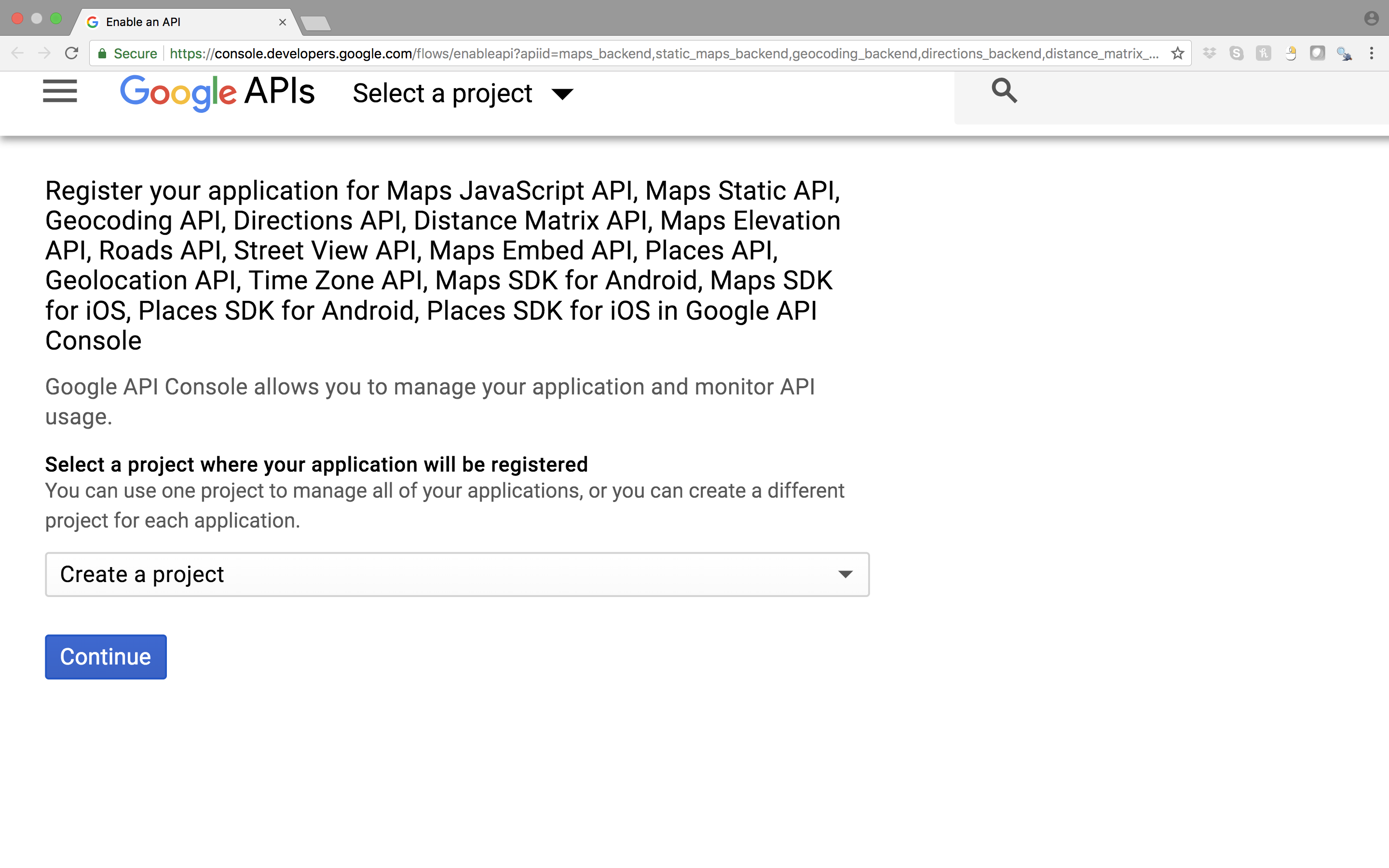
Click the continue button under the dropdown menu “Create a Project”. It will take a while to load, but you’ll see this screen:

Type whatever name you like, but make sure to specify “HTTP referrers” as one of the application restricters. Include afterwards (localhost:*) to be one of the request locations so you won’t get blocked when running this in your console.
Afterwards, make sure to copy your key and leave it somewhere so you can remember. I’ll just store it here as a vector. You’ll need this key for any google project you’ll be focused on!
key <- "AIzaSyByzQkHPZtdoCRRBxAeQL48hsZJLz8cPLs"
The great thing about accessing the Google API service is how you not only have the maps service, but a plethora of other utilities: translate, adsense, shopping, and other API tools that Google allows for the public.
I personally use the translate API pretty often in this workplace. Usually it’s only to translate vectors of industry information from Japanese to English or vice versa, but I seem to use it more often then naught (I enjoy the direct translation and ease a lot better than the Microsoft API that’s accessible through most R packages).
Now that we have our key, let’s get started!
Data comes from AggData and displays locations for all US public libraries with variables such as: Name, address, phone number, and latitude/longditude.
The only package we’ll really need is the plotGoogleMaps package. This allows for the recognition of our API authentication and access to the google maps dashboard. For convenience purposes, I’ve also installed the tidyverse packages.
library(plotGoogleMaps)
library(tidyverse)
Next, let’s take a glimpse of the dataset that we have here.
link <- "https://www.aggdata.com/download_sample.php?file=public_libraries.csv"
libs <- read_csv(link)
glimpse(libs)

It seems like we have some good information giving us the location, location type, position, and state. Let’s filter out some of these variables.
keep <- c(2:8,10:11)
bibliotecas <- libs[keep]
bibliotecas$`Location Type` %>% unique
table(bibliotecas$`Location Type`)
##  Bookmobile  Branch Library Central Library  Library System
##         635            7644            9040            9207
Now that we’ve set aside our data, let’s just say that we had a hypothetical case where we worked for the “Librarian of Congress” for this year (yes, this position actually exists. And also yes, this is probably not the situation you were looking for but I had to find some reason to show this). As your duty to make sure that all the “U.S. Poet Laureates” are recognized in every Bookmobile, you have been to hunt down the location of all the Bookmobiles to negotiate with them a plaque for this years award winner. Of course, she cannot visit all 635 locations, so she has to choose wisely which places in the US have the highest density of Bookmovies and take a trip there. The rest will sadly have to do with a letter of request.
Let’s first subset our dataset and take a look at the distribution of Bookmobiles by state
sub <- subset(bibliotecas,bibliotecas$`Location Type` == "Bookmobile")
table(sub$State) %>% as.vector %>% hist
table(sub$State) %>% as.vector %>% summary

## Min. 1st Qu.  Median    Mean 3rd Qu.    Max.
##  1.0     3.0     8.0    12.7    17.5    74.0
With a skewed distribution, it’s safer to say that the median is the best statistic we could use to describe our population.
We’ll now subset to the states that have larger than normal counts of central libraries so she can hit multiple targets at once.
ind <- table(sub$State) > 8
use <- table(sub$State)[ind] %>% names
min <- subset(sub,sub$State%in%use)
Now that we’ve chosen the states, let’s map these out! The only information we really need is the lattitude and longditude information. This may be a little unfortunate as we end up losing precious information. Yet, we have to melt the table to fit the coordinate system. By using coordinates() we initially take the variables lon and lat and change them to coordinates, but take another step and convert the longditude and latitude coordinates into state plane coordinates by using the CRS("+init=epsg:4326") command. Make sure to be exact as this is the string that identifies the correct state plane coordinates.
lonlat <- min[,c(9:8)]
lonlat <- as.data.frame(lonlat)
names(lonlat) <- c("lon","lat")
# into coordinates, then state plane coordinates.
coordinates(lonlat) <- ~lon+lat
proj4string(lonlat) <- CRS("+init=epsg:4326")
At first, I tried just pasting in the api key that I received from google, but it wasn’t working. After a bit of searching, I found out that it had to be under a certain URL with the key attached. All we need to do is paste that in here. Also, by specifying the ‘gets b’ b <- is actually pretty important here. It can be anything, but we want to make sure to avoid getting flooded by the html version of what you plot.
api <- "https://maps.googleapis.com/maps/api/js?libraries=visualization&key="
apikey <- paste(api,key,sep = "") # combine key and site location.
b <- plotGoogleMaps(lonlat, api = apikey)

This is actually pretty comical as it doesn’t really explain anything, but it is a rather useful tool in getting a good snapshot view of what you’re looking for. It seems like the most populated locations are in Kentucky, California, Ohio, and South Carolina. They seem to be the most dense and closely packed. Now your manager is happy and you are good to go (:.
I am definitely sure there are more useful procedures we can deal with especially if we are getting into deeper cluster or geospatial analysis. This is just more of me exploring what I can produce with R! I’ll be exploring more as time progresses. I hope you enjoyed the short demonstration!