Who buys what and what with what? … What?
Association mining is a simple, yet expensive task. Being inundated in data, it isn’t easy to string things together.
The whole goal here is to find a technique that will efficiently grab the frequencies of basket items. Let’s give this a try. Fortunately, we have R. Though MLxtend in python is much faster in some ways, it cannot make useful infographics or parse redundant rules.
For this post, we will be using the apriori algorithm to do a market basket analysis.
In the most simplest of senses, the apriori algorithm is a technique to determine a minimum frequency threshold to parse out data that is unnecessary. If an itemset is frequent, we assume that all of its subsets are also frequent. This is called an ‘anti-monotone’ property of support. Support in this sphere means frequency. The assumption states that the support of the individual item never exceeds the support of its subsets. If one parent is found to be infrequent, everything beneath it will also be infrequent.
For more information on apriori, read this example. It will be very useful.
For bigger datasets, it may be in our favor to use a PCY or SON algorithm, however, our store we are dealing with only has 10 items. No need to worry.
Let’s get started!
We have a small store that sells about 20 objects. We are heavily interested in what people like to buy when they buy certain items. Let’s take a look at some association rules. Make sure to install the packages: arules and arulesViz to run our apriori algorithms. These packages can also handle brute force and sampling algorithms, however let’s try the most common and intuitive.
library(tidyverse)
library(arules)
library(arulesViz)
As we read in our data, you might want to take a look at the way the information is structured. A good way to mutate the data to fit this form has been found on datacamp. If you have a pre-made dataset, just use this code below and your transactions data should be read in.
transactions.data <-as(data,"transactions")
datapath <- "https://raw.githubusercontent.com/tykiww/projectpage/master/datasets/Market-Basket/mbb.csv"
mba <- read.transactions(datapath, format = 'basket', sep = ',')
summary(mba)
As you read in the data, you may get an error that says..
## incomplete final line found on '~/mbb.csv'
Ignore it for now. We will do something to fix those later.
Our summary prints:
## Transactions as item Matrix in sparse format with
##  3001 rows (elements/itemsets/transactions) and
##  3011 columns (items) and a density of 0.001307989
##
## most frequent items:
##   bread  cheese    beer diapers burgers (Other)
##    3000    1496    1044     777     557    4945
## ...
We notice 3001 collection of items and 3011 different items. This 3011 includes unique combinations, which indicates we may not have very much use of our data. However, we will still be able to proceed.
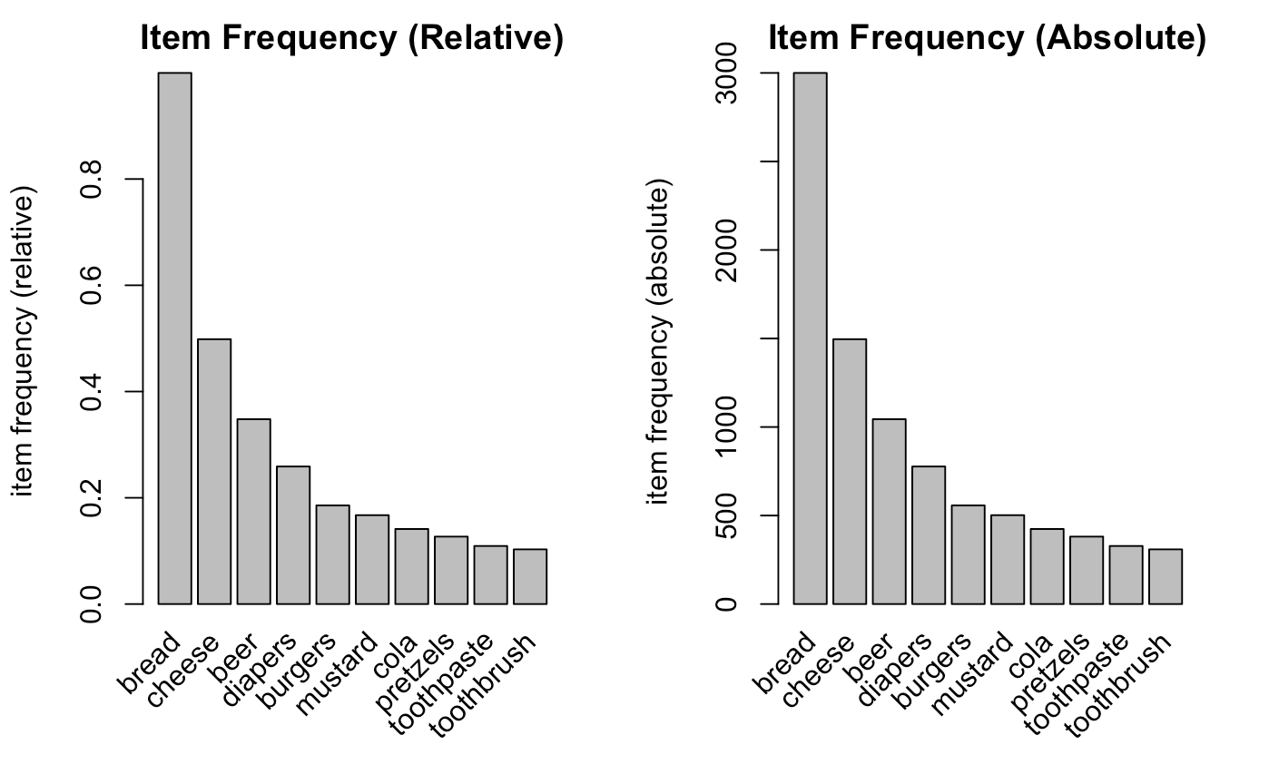
Now plotting an item support plot, we notice that bread is bought the most with the toothbrush least.
par(mfrow = c(1,2))
# Relative will plot how many times these items have appeared as compared to others %.
itemFrequencyPlot(mba,topN = 10,type = "relative", main = "Item Frequency (Relative)")
# Absolute will plot numeric frequencies of each item independently.
itemFrequencyPlot(mba,topN = 10,type = "absolute", main = "Item Frequency (Absolute)")
par(mfrow = c(1,1))
Moving on to our model, we will use the function apriori() to fit our data with some parametrs. The most important ones are:
- minimum support : Support(B) = (Transactions containing (B))/(Total Transactions)
- minimum confidence : Confidence(A→B) = (Transactions containing both (A and B))/(Transactions containing A)
- minimum length : Defining the minimum length of items in a transaction
I am looking to find itemsets or rules that occur at least 5 times, so I will divide 5 by the length of entire dataset. As for minimum confidence, we will first begin with 0, and find the best value after running our initial model. Transactions with a single item will not explain anything from our data, therefore we will keep our minimum length at 2.
minsup <- 5 / length(mba) # I want to find itemsets/rules that occur at least 5 times.
minconf <- 0 # init.
minlen <- 2 # Take out single items.
params <- list(supp = minsup, conf = minconf, minlen = minlen, target = "rules")
Fitting our model will display a small screen of our data.
ar <- apriori(mba, parameter = params) # Lift(A→B) = (Confidence (A→B))/(Support (B))
inspect(tail(ar, by = "confidence"))
##     lhs                            rhs          support     confidence lift      count
## [1] {diapers,mustard}           => {toothbrush} 0.002665778 0.06250000 0.6069984 8
## [2] {bread,diapers,mustard}     => {toothbrush} 0.002665778 0.06250000 0.6069984 8
## [3] {beer,cheese,mustard}       => {toothbrush} 0.001666111 0.05952381 0.5780937 5
## [4] {beer,bread,cheese,mustard} => {toothbrush} 0.001666111 0.05952381 0.5780937 5
## [5] {burgers,mustard}           => {toothbrush} 0.001666111 0.05263158 0.5111565 5
## [6] {bread,burgers,mustard}     => {toothbrush} 0.001666111 0.05263158 0.5111565 5
Now we see a lift metric above. Lift is calculated as: Lift(A→B) = (Confidence (A→B))/(Support (B)). The higher the lift, the more meaningful as it denotes less of a coincidence. Before we interpret the information, let’s find our lowest threshold for confidence.
tail(ar, by = "confidence") %>% inspect
##     lhs                            rhs          support     confidence lift      count
## [1] {diapers,mustard}           => {toothbrush} 0.002665778 0.06250000 0.6069984 8
## [2] {bread,diapers,mustard}     => {toothbrush} 0.002665778 0.06250000 0.6069984 8
## [3] {beer,cheese,mustard}       => {toothbrush} 0.001666111 0.05952381 0.5780937 5
## [4] {beer,bread,cheese,mustard} => {toothbrush} 0.001666111 0.05952381 0.5780937 5
## [5] {burgers,mustard}           => {toothbrush} 0.001666111 0.05263158 0.5111565 5
## [6] {bread,burgers,mustard}     => {toothbrush} 0.001666111 0.05263158 0.5111565 5
We see here that our minimum confidence is 5.2%. Of course with larger datasets, minconf can be a method to parse out values that have a small percentage of measures that appear in one transaction relative to another object. It seems like there is a good spread of transactions occur with each other. Also, since we are using R, lets go on and remove the redundant variables for our improved model.
# adapt confidence
minconf <- .05
ar <- apriori(mba, parameter = params)
# remove redundant.
a <- ar[!is.redundant(ar)]
inspect(a)
##       lhs                                    rhs          support     confidence lift      count
## [1]   {toothbrush}                        => {toothpaste} 0.011329557 0.11003236 1.0067290   34
## [2]   {toothpaste}                        => {toothbrush} 0.011329557 0.10365854 1.0067290   34
## [3]   {toothbrush}                        => {pretzels}   0.012662446 0.12297735 0.9686483   38
## [4]   {pretzels}                          => {toothbrush} 0.012662446 0.09973753 0.9686483   38
## [5]   {toothbrush}                        => {cola}       0.012329224 0.11974110 0.8475072   37
Let’s now interpret our model. Those who buy a toothbrush tend to buy toothpaste and vice versa. The lift is above 100% which indicates that this rule is very likely to be true. However, only 11% of transactions dealing with toothpaste and toothbrush corresponded with overall toothpaste sales.
If we were to visualize the 15 most important rules..
spected <- head(a, by = "confidence",15)
plot(spected, method = "graph",  engine = "htmlwidget")

We can play around with the different rules and products. The most connected rule leads to bread. It makes sense as the most ubiquitous. Play around with the widget and see what you can discover.
If we were interested in a particular product relative to the others, we may reverse engineer the process. How about diaper buyers?
apps <- list(default = "rhs", lhs = "diapers")
diapers.ar <- apriori(mba, parameter = params, appearance = apps)
inspect(diapers.ar)
##     lhs          rhs          support    confidence lift      count
## [1] {diapers} => {toothbrush} 0.02465845 0.0952381  0.9249499  74
## [2] {diapers} => {toothpaste} 0.02765745 0.1068211  0.9773480  83
## [3] {diapers} => {pretzels}   0.03198934 0.1235521  0.9731757  96
## [4] {diapers} => {cola}       0.03565478 0.1377091  0.9746819 107
## [5] {diapers} => {mustard}    0.04265245 0.1647362  0.9848072 128
## [6] {diapers} => {burgers}    0.04798401 0.1853282  0.9985097 144
## [7] {diapers} => {beer}       0.08930357 0.3449163  0.9914693 268
## [8] {diapers} => {cheese}     0.12295901 0.4749035  0.9526640 369
## [9] {diapers} => {bread}      0.25891370 1.0000000  1.0003333 777
Diaper buyers who bought Bread were represented in all diaper transactions. Furthermore, Cheese seemed to be another important product as well.
What about purchases that were made in association with cheese?
apps <- list(default = "lhs", rhs = "cheese")
cheese.ar <- apriori(mba, parameter = params, appearance = apps)
inspect(head(cheese.ar,5, by = "confidence"))
##      lhs                                         rhs      support     confidence lift     count
## [1] {burgers,diapers,mustard,pretzels}       => {cheese} 0.001666111 1.0000000  2.006016  5
## [2] {bread,burgers,diapers,mustard,pretzels} => {cheese} 0.001666111 1.0000000  2.006016  5
## [3] {mustard,pretzels,toothpaste}            => {cheese} 0.001666111 0.8333333  1.671680  5
## [4] {bread,mustard,pretzels,toothpaste}      => {cheese} 0.001666111 0.8333333  1.671680  5
## [5] {diapers,mustard,pretzels}               => {cheese} 0.003665445 0.7857143  1.576155 11
Cheese seemed to be highly associated with the above combinations.
In the end, we should remember that practical datasets will involve larger volume and much specific metrics (gini, J-measure, mutual info, etc.). In certain contexts, even confidence will not work as the best metric with the possibility of underestimating indicidual characteristics. Furthermore, we must choose carefully our metrics whether the data is dependent or independent.
Regardless, here is another device for your toolkit. Have fun with it!