
Dimension Reduction is a technique necessary to have for almost any high-dimension analysis. In short, Principal Component Analysis is a technique to reduce dimensionality (essentially variables) and make data easier to interpret. It’s really easy (even if you don’t have any linear algebra experience, though it definitely helps) and can improve any covariate analysis.
PCA can be done in four simple steps:
- Calculate the Covariance/Correlation matrix.
- Calculate the eigenvectors and the eigenvalues of the covariance matrix.
- Create our new dataset and select the principal components to use.
- Analyze our set
Also, PCA has the following assumptions:
- Data must be numeric. Sometimes, you can use dummy variables, but it always depends.
- PCA is sensitive to outliers and should be removed
- Assumes the presence of relatedness between the variables
Let’s do some PCA using some credit info on ethnicities (just for fun, I didn’t create this set). What ethnicity would I be given a certain set of characteristics?
library(tidyverse)
"https://raw.githubusercontent.com/tykiww/projectpage/master/datasets/credit/Credit.csv" %>%
  read_csv -> credits
Cleaning
Before we get into the PCA, let’s clean our dataset real quick. All of our binomial categorical variables will be dummied as 0,1 and our ethnicity variable will be removed for now.
credits$Gender <- ifelse(credits$Gender == "Male",0,1)
credits$Student <- ifelse(credits$Student == "No",0,1)
credits$Married <- ifelse(credits$Married == "No",0,1)
Standardizing and validating the data is also important if prediction is at hand.
Standardizing the data with mean 0 and variance 1 allows for measuring columns of different scales. This is especially useful because PCA creates a feature space that maximizes the variance along the axes. However, this makes for interpretation to be a bit difficult. If you are to standardize, make sure to re-transform the data back afterwards! For this analysis, we will not be scaling just to make things a bit simpler to explain. We will also make sure to grab a test dataset just to help us with our predictions.
# caret::scale(credits[,-c(1,11)])
idx <- sample(nrow(credits),round(.8*nrow(credits), digits = 0), replace = FALSE)
credits_trn <- credits[idx,-c(1,11)]
credits_val <- credits[-idx,-c(1,11)]
Step 1: Calculate the Covariance/Correlation matrix.
This step is only one line of code. However, let’s talk about the importance of the covariance/variance matrix. A variance/covariance matrix is a matrix where each element represents the covariance between two features. The diagonal elements of the matrix contain the variances of the variables (which will be 1 for a normalized dataset) and the off-diagonal elements contain the covariances between all possible pairs of variables. “Covariance” indicates the direction of the linear relationship between variables. “Correlation” on the other hand measures both the strength and direction of the linear relationship between two variables. We can take a glimpse of the matrix to see the covariances between all possible pairs of variables in the data set.
(cred_cov <- cov(credits_trn))
##                  Income         Limit        Rating        Cards           Age     Education        Gender     Student      Married
## Income     1296.1485505  6.812713e+04  4.565508e+03 -0.468889773  129.98033342   5.918122571  -0.270234855  0.67139477  0.529618828
## Limit     68127.1259872  5.633103e+06  3.770343e+05 49.793025078 4880.24506270 221.092789969 -25.681857367  7.15544671 24.343064263
## Rating     4565.5083650  3.770343e+05  2.538576e+04 12.377684169  336.75197884  11.868181818  -1.637176724  0.83406152  2.180887539
## Cards        -0.4688898  4.979303e+01  1.237768e+01  1.803722571    1.30654389  -0.167084639  -0.007229624 -0.01052116 -0.001665361
## Age         129.9803334  4.880245e+03  3.367520e+02  1.306543887  298.29776646  -0.523197492   0.074902038 -0.32525470 -0.371571317
## Education     5.9181226  2.210928e+02  1.186818e+01 -0.167084639   -0.52319749   9.464576803  -0.003605016  0.04717868  0.082288401
## Gender       -0.2702349 -2.568186e+01 -1.637177e+00 -0.007229624    0.07490204  -0.003605016   0.250303683  0.01198080  0.003869514
## Student       0.6713948  7.155447e+00  8.340615e-01 -0.010521160   -0.32525470   0.047178683   0.011980799  0.08776450 -0.012196317
## Married       0.5296188  2.434306e+01  2.180888e+00 -0.001665361   -0.37157132   0.082288401   0.003869514 -0.01219632  0.238783307
## Balance    8284.3876097  9.699550e+05  6.539306e+04 53.903350313    6.60366379  15.543730408  -1.899422022 33.84062500 -3.766702586
##                 Balance
## Income      8284.387610
## Limit     969954.959365
## Rating     65393.064743
## Cards         53.903350
## Age            6.603664
## Education     15.543730
## Gender        -1.899422
## Student       33.840625
## Married       -3.766703
## Balance   218968.056025
From this figure we notice that Married and Gender have the least amount of relationship (most independent, closest to 0) and credit limit with credit rating have a higher relationship. These both seem to make sense as married and gender are bivariate columns yielding a small amount of information whereas the credit limit and ratings seem reasonable to increase together to a certain extent.
Step 2: Calculate the eigenvectors and the eigenvalues of the covariance matrix.
Now we will go on to finding our eigenvectors and eigenvalues. In short, eigenvectors represent our “principal components” which determine the direction of the new feature subspace. Eigenvalues on the other hand determine the magnitude of each eigenvector. The code eigen() will take care of this. If you are curious on how to compute these values, take a look at this resource.
(eigen(cred_cov) -> vecs)
## eigen() decomposition
## $values
##  [1] 5.827681e+06 5.070197e+04 2.922802e+02 2.439952e+02 1.324867e+02 9.362627e+00 1.247117e+00 2.508287e-01 2.300412e-01 3.359181e-02
##
## $vectors
##                [,1]          [,2]          [,3]          [,4]          [,5]          [,6]          [,7]          [,8]          [,9]         [,10]
##  [1,] -1.178894e-02 -6.953288e-02 -0.4239469805  0.8500518501  0.3040377668 -0.0112575167 -0.0016768874  7.175011e-04 -0.0023968096  0.0114996900
##  [2,] -9.830364e-01 -1.697654e-01  0.0270157744 -0.0334928114  0.0543105516 -0.0013193559 -0.0039958761 -1.830549e-04 -0.0003407178 -0.0003516326
##  [3,] -6.581203e-02 -2.227399e-03 -0.2113129291  0.2319689523 -0.9450511502  0.0223257013  0.0594217328  2.344587e-03  0.0066555525 -0.0004661131
##  [4,] -1.011802e-05  8.779319e-04 -0.0151694160  0.0112464957 -0.0566741613  0.0036592273 -0.9971304106 -2.024496e-02 -0.0257413692 -0.0327986498
##  [5,] -8.275208e-04 -1.650262e-02 -0.8791925405 -0.4690691751  0.0818261360  0.0031497073  0.0034721408  7.896045e-05 -0.0019985713  0.0002665135
##  [6,] -3.789632e-05 -4.475140e-04  0.0027873189  0.0057694911  0.0246016499  0.9996164227  0.0018681971  2.042952e-03  0.0098932086  0.0038689852
##  [7,]  4.406808e-06  4.958759e-05 -0.0007604681  0.0005181565  0.0001469934 -0.0002246677  0.0133124255 -9.774814e-01  0.2074929099  0.0360365796
##  [8,] -2.209487e-06  6.312103e-04 -0.0046322525  0.0092959288  0.0060497983  0.0034182660  0.0326396384 -3.079996e-02  0.0261969247 -0.9985705697
##  [9,] -4.021544e-06 -1.552304e-04  0.0015476873  0.0005679174 -0.0054441168  0.0102387559  0.0303816276 -2.077531e-01 -0.9774689803 -0.0182422496
## [10,] -1.707882e-01  9.828867e-01 -0.0405477094  0.0469874643  0.0301785617 -0.0004695039  0.0002588267  8.107698e-05 -0.0004010508  0.0014238541
The eigenvalues are ordered in descending order. The first component (5.51) is larger than the second component, and continues to descend in importance. The highest will be the ones to keep, but we will have to determine that next.
Step 3: Create our new dataset and select the principal components to use.
The new dataset can be calculated with ease. It is the transposed matrix of the vectors times the transposed matrix of the scaled dataset transposed all together.
# The new dataset
pr_credit <- t( t(vecs$vectors) %*% t(credits_trn))
colnames(pr_credit) <- sapply(seq(1,ncol(credits_trn)),
                              function(x) paste("PC",x, sep = ""))
pr_credit
##               PC1         PC2        PC3         PC4       PC5       PC6           PC7           PC8        PC9       PC10
##  [1,]  -8138.4424 -182.813015 -39.178146 -38.8469376 -66.94854 17.601797  0.9739784221 -0.1470836852 -0.4152044 -0.5973150
##  [2,]  -2076.8486 -359.202695 -43.022482 -48.0362403 -37.27931 15.079560 -0.0023831736  0.0205865342  0.3425658 -0.6360273
##  [3,]  -3828.8183 -664.258312 -26.332882 -15.6416315 -44.77592 14.837750 -0.6779795750 -1.1704943022 -0.3079567 -0.6494896
##  [4,]  -1552.2279 -268.062122 -36.883413 -27.2308632 -60.73561 20.593399 -1.4172554757 -0.1660405933 -0.4918934 -0.5999897
##  [5,]  -2532.2241 -438.725399 -25.436987 -17.4922752 -48.33814 15.080671  0.6600834096 -0.1518117928 -0.5032578 -0.5447375
##  [6,]  -2125.4375 -369.341611 -61.014640 -33.6769474 -28.55413 15.830493 -2.0768550517 -0.0043020841  0.2206535 -0.4399971
##  [7,]  -4954.9406 -558.502739 -20.780840 -38.3383388 -44.22338 13.940849  1.0599560899 -1.1613351226 -0.2828576 -0.7597325
##  [8,]  -4385.9073  -76.499990  -7.290024 -37.2388251 -46.61784 17.201863 -2.5779053214 -1.2142965142 -0.3964450 -0.6322562
##  [9,]  -4464.6828 -315.118194  -4.266436 -42.4494808 -31.81683 14.733168  0.2395481391 -0.9806852782  0.5966016 -0.6532897
## [10,]  -5161.2288 -171.822535 -37.297495 -55.5729459 -49.21962 20.369263 -0.2712760228 -0.9562991952  0.6512964 -0.6322667
## ...
Now, in order to decide which eigenvectors should dropped without losing too much information we will inspect the magnitude of the eigenvalues. The eigenvectors with the lowest eigenvalues explain the least variance about the distribution of the data; those will be dropped. This can be done by just a simple for loop and finding the cumulative percentages of the eigenvectors.
sapply(vecs$values, function(x) 100 * (x/sum(vecs$values)) ) %>% cumsum
The first principle component already explains 99% of the data. For the most case, the 1st and 2nd principle components always explain over 40% of the data. Keeping the first two components will be enough to map our data.
Is there an easier way?
Yes. There is always a better, faster way. Let’s take a look at everything we did in one step below using the base R prcomp function.
library(ggfortify)
prcomp(credits_trn) %>%
  autoplot(data = mutate(credits_trn,'Ethnicity' = credits$Ethnicity[idx]), colour = 'Ethnicity',
           loadings = TRUE, loadings.label = TRUE,
           x = 1, y = 2)
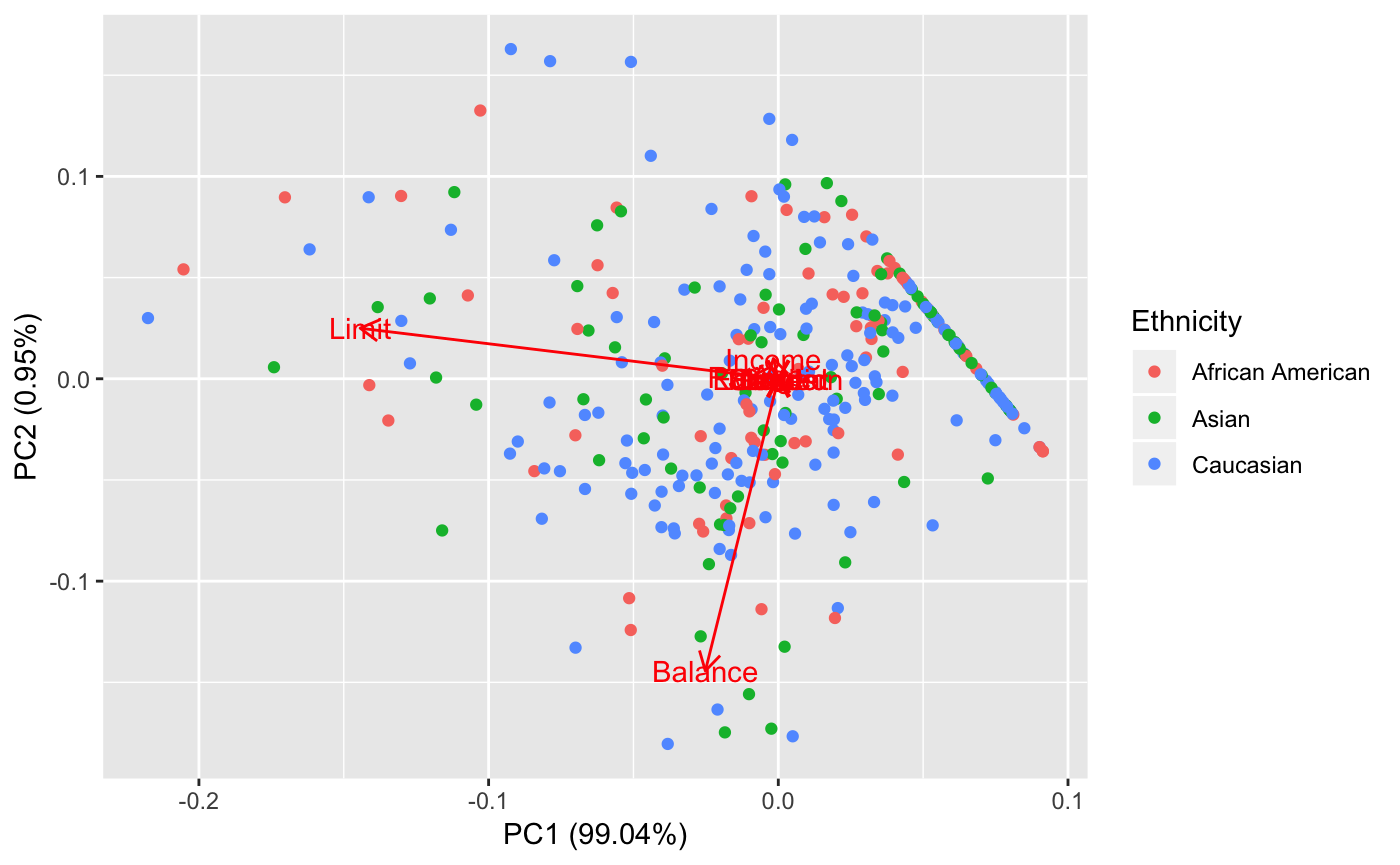
We see that the data is difficult to compartamentalize. There are no simple clusters seen here. However, we notice that the first principal component is heavily relied on credit limit. We notice here that having 99% of the data explained in the first principal component is not necessarily ideal for interpretation. This indicates that most of our indicators are pretty bogus OR, there really is no general difference between ethnicities in terms of the original profiling covariates.
However, let’s try running some predictive modeling. Maybe some recursive partitioning? We will compare the principal component recursive partions with the dataset without any partitioning.
library(rpart)
prin_comp <- prcomp(credits_trn) # training
dat_mod <- data.frame(Ethnicity = credits$Ethnicity[idx], prin_comp$x[,1:2])
rpart_model <- rpart(Ethnicity ~ .,data = dat_mod, method = "class")
rpart_no <- rpart(Ethnicity ~ ., data = mutate(credits_trn,'Ethnicity' = credits$Ethnicity[idx]), method = 'class')

# Test Prediction
test_data <- predict(prin_comp, newdata = credits_val) %>% as_tibble
#make prediction on test data
pred_item <- predict(rpart_model, test_data[,1:2])
pred_no <- predict(rpart_no, credits_val)
## PCA      African American   Asian  Caucasian   None    African American   Asian  Caucasian
##  1         0.1250000 0.1666667 0.7083333      1         0.8571429 0.00000000 0.1428571
##  2         0.1769912 0.2566372 0.5663717      2         0.1492537 0.17910448 0.6716418
##  3         0.1769912 0.2566372 0.5663717      3         0.3333333 0.19047619 0.4761905
##  4         0.1769912 0.2566372 0.5663717      4         0.1363636 0.22727273 0.6363636
##  5         0.1250000 0.1666667 0.7083333      5         0.2000000 0.60000000 0.2000000
##  6         0.1769912 0.2566372 0.5663717      6         0.0000000 0.70000000 0.3000000
##  7         0.1769912 0.2566372 0.5663717      7         0.1111111 0.33333333 0.5555556
##  8         0.1769912 0.2566372 0.5663717      8         0.1333333 0.00000000 0.8666667
##  9         0.4210526 0.2631579 0.3157895      9         0.5882353 0.11764706 0.2941176
##  10        0.1769912 0.2566372 0.5663717      10        0.0000000 0.23809524 0.7619048
Now taking a look at our probability matrix, we can make a comparison by taking the item with the highest probability and doing a 1-1 comparison. We can definitely do better, but just for simplicity sake.
# Nothing
scored_no <- sapply(1:nrow(pred_no), function(x) names(which.max(pred_item[x,])))
mean(scored_no==credits[-idx,]$Ethnicity)

# PCA
scored_pc <- sapply(1:nrow(pred_item), function(x) names(which.max(pred_item[x,])))
mean(scored_pc==credits[-idx,]$Ethnicity)
## [1] 0.425
## [1] 0.425
The model itself is not so great, but the power to explain our data is practically the same. Isn’t that cool? Just so you don’t freak out, it was only by chance that both the pca data and the non-transformed data performed exactly the same. However, it has to be very close. Now think of having to work with a huge dataset with multiple columns of covariates? Wouldn’t this make computation so much simpler? Next time you have a dataset with large amounts of columns, consider using some dimension reduction techniques.