Date manipulation can be a pain. Sometimes, this is due to the random formatting of different dates. In my personal opinion, R has quite a terrible class for dates. It MUST include year, month, and day. If not, you have to make sure to use format() to coerce it to a Year-month, Year-day combination. I looked online for some other classes. The zoo package apparently has a yearmon class. Yet, we don’t necessarily need that. It seems like a convenience issue. I believe it should be standard practice to separate out the Overall date, Year, Month, and Day for every raw dataset. I guess that’s just wishful thinking.
For example, the other day, I was doing a BI analysis for an HR risk company. I was just investigating some of their data to see if I could extract any useful information. Unfortunately, there wasn’t much from what I got to inference anything. I was, however, able to pull out the number of days each employee had been working. During that process, I remembered again how lack of date standardization can be a pain.
Today, I’ve pulled out some cleaner date data to show you some simple ways to manipulate dates effectively for useful analysis. After I clean it to what I want, I’ll use it for a regression analysis.
Here are the packages to load for this post. I don’t think I ever used tidyr for any of my posts. Probably one of the most prized out of all data cleaning packages. They have a goal to clean data to make it as readable as possible. Various shortcut techniques allow us pull and push together columns easily, pivot and reorder columns. Other packages actually fall under what is called the ‘tidyverse’ which already include ggplot2,dplyr,readr (reading in datasets), and many others. Technically, all I need to do is just load the tidyverse library and it will all give me what I want. I might start doing that, but it’s always nice to know what each item is coming from.
library(tidyr)
library(tidyverse) # Do this instead for more packages
The data comes from my github repository. I got the first file from the utah avalanche center and downloaded avalanches from all regions in Utah. The second, I had to order from an airport. The information is sorted on a government site and allows you to extract information and send it to your email. I have the Salt Lake City international airport weather data. I decided to use read_csv() information form readr package. Not much is different for now. It’s probably because the columns are already rather clean. One plus is definitely the information output you get of the NAs that appear. Always nice to have extra information.
ava <- read_csv("http://tykiww.github.io/assets/Poisson/reco-download.csv", col_names = T)
cli <- read_csv("http://tykiww.github.io/assets/Poisson/1299199.csv", col_names = T)

Alright, now for the dates. There was actually a lot more scrubbing that had to be done previously, but here is what I did. R doesn’t automatically recognize dates pretty often, so you have to coerce it using as.Date(). Make sure to format it correctly with "%m/%d/%Y". I also used the substr function to cut out the date variables. We are only looking at the year and month
# Create date elements for climate and avalanche
ava$Date <- ava$Date %>%
  as.Date("%m/%d/%Y")
ava$Date <- ava$Date %>%
  substr(1,7)
cli$DATE <- cli$Date %>%
  as.character()

ava <- ava[,-(5:9)] # Remove ignore columns
The aggregate() function comes in very handy if you are trying to use a function over a certain value of factors. Interestingly, this functions very similarly to tapply over the Date variables. One advantage the aggregate function has over tapply is that it spits out a dataframe rather than an array. The dataframe will make it easier to just stick it back into our original data.
Also, avalanches aren’t too big of a problem outside of winter months, so we will get rid of every month except December, January, Februrary, and March. I used the | operator again just like in the credit card post to extract those exact months.
# Counting up number of avalanches per month
t <- aggregate(Nid ~ Date, FUN = length, data = ava)
# only winter months
t <- t[grepl("-12|-01|-02|-03",t$Date),]
cli <- cli[grepl("-12|-01|-02|-03",cli$DATE),]
Next is inserting the frequency of avalanches into the original cli dataset. This part took a little bit of thinking, but it all worked out. I used the %in% operator to find out the dates that correspond with the t dataset, and created an empty row to insert it in. I then found the dates inside the t dataset that corresponded with the climate date and stuck those back in.
Afterwards, I used the tidyverse function separate() to split the Date. It’s really simple as long as you do have a valid separator. I once worked with information with some separators and some without. It gets really annoying especially with rows greater than 1000. Now the dates are readable and useful in any case!
cli$count <- 0 # create empty column
cli$count[cli$DATE %in% t$Date] <- t$Nid[t$Date %in% cli$DATE] # match insert
dates <- cli$DATE
cli <- separate(cli,DATE, c("Year","Month") ,sep = "-")
avalanches <- cbind(cli,dates)
rm(cli,ava,t) # we have what we need.
glimpse(avalanches)
## Observations: 74
## Variables: 8
## $ STATION <chr> "USW00024127", "USW00024127", "USW00024127"....
## $ Year    <chr> "2000", "2000", "2000", "2000", "2001", "20....
## $ Month   <chr> "01", "02", "03", "12", "01", "02", "03", "....
## $ DT32    <int> 20, 16, 17, 30, 31, 23, 12, 29, 30, 27, 17,....
## $ SNOW    <dbl> 15.0, 5.1, 6.2, 12.9, 6.6, 13.1, 5.3, 20.0,....
## $ TMIN    <dbl> 27.4, 31.1, 32.0, 22.9, 21.2, 26.5, 35.8, 1....
## $ count   <dbl> 1, 0, 0, 1, 0, 1, 1, 0, 1, 0, 1, 0, 0, 1, 0....
## $ dates   <fct> 2000-01, 2000-02, 2000-03, 2000-12, 2001-01....
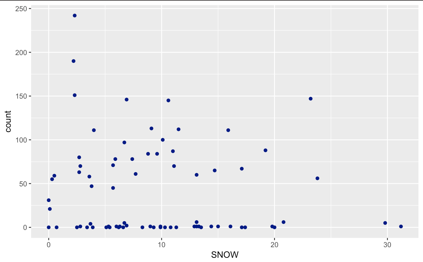
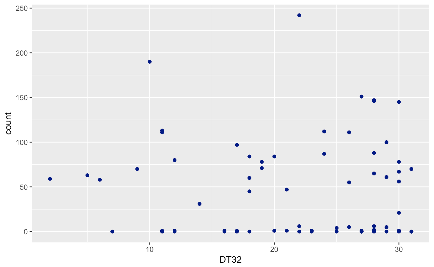
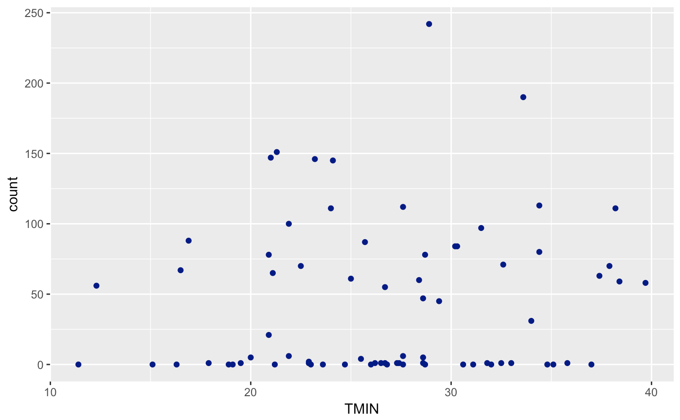
Let’s create a scatterplot of Avalanches (count) and each useful variable (SNOW, TMIN, DT32). As you can see, I’m trying to milk as much of the tidyverse as possible with limited range. I won’t be able to cover all packages though.
ggplot(avalanches, aes(SNOW,count)) + geom_point(col = "dark blue")
ggplot(avalanches,aes(DT32,count)) + geom_point(col = "dark blue")
ggplot(avalanches,aes(TMIN,count)) + geom_point(col = "dark blue")
If you look very carefully, you’ll notice that the variables are not technically continuous, but discrete. You can’t have .5 avalanches, neither can you have negative avalanches. Usually, we can perform a regular regression with this data and it will be fine for this case. Yet, we run into a problem when we try and assume that the errors are normally distributed. Unfortunately, the errors cannot go below 0. Therefore, we will have a non-normal error distribution. Let’s take it a step further and use an already-known distribution for this data!
The model will use a Poisson distribution. A poisson is defined as “a discrete probability distribution that expresses the probability of a given number of events occurring in a fixed interval” - Wikipedia. Well said. Number of Avalanches occuring in a fixed interval. We wouldn’t be able to use something like a hypergeometric or binomial as we are not sampling from a number of trials. It is the probability of the average number of times an avalanche occurs in a fixed interval.
The model in R already takes into account a log transformation. A log transformation looks useful because we have an increasing variance as the number of avalanches goes up. Fortunately, the glm package takes care of it. The “Link” function inside embeds the log transformation inside the maximum likelihood estimation.
Written out, the model looks something like this.
Model: y ~ Poisson(exp(Bo + B1(SNOW) + B2(TMIN) + B3(DT32)))
It’s not much different from a linear regression. Actually, an old method was to use a square root transformation of count and taking a linear regression. The square root, (since the data never goes to zero) accounts for variation inflation and other annoying factors. Let’s not do that though. We already have a known distribution.
out.avalanche <- glm(count ~ SNOW + TMIN + DT32, data = avalanches, family = "poisson")
summary(out.avalanche)
## Coefficients:
##              Estimate Std. Error z value Pr(>|z|)
## (Intercept)  3.646778   0.317161  11.498  < 2e-16 ***
## SNOW        -0.023612   0.003373  -7.001 2.54e-12 ***
## TMIN         0.009802   0.007199   1.361    0.173
## DT32         0.002713   0.005667   0.479    0.632
The coefficients for this data are:
snow - The average count of snowfall by month and year. TMIN - The monthly minimum temperature by each month and year. DT32 - The average number of days below 32 degrees by each month and year.
We see a negative coefficient in our snowfall and avalanche beta value. This is hard to imagine, but it looks like when snowfall increases, the count of avalanches decreases. After looking up a little more information on snowfall patterns we can see that periods of high snow accompanied by long length without snow may be the cause for avalanches. There is an odd pattern of snowfall that the model IS capturing. This is an unusual finding as variable patterns of snowfall seem to be the case for increased avalanches.
For the effect of Temperature on the mean number of avalanches, we can say that with a p-value of (0.173) we can fail to reject the null hypothesis and say that there is not a statistically significant effect of minimum monthly temperature on the number of avalanches.
Then, for the effect of number of days below 32 degrees, with a p-value of (0.632), we fail to reject the null hypothesis that there is no effect of in number of days below 32 degrees on the number of avalanches.
Now notice that the summary coefficient outputs are still in the natural log state. For clear interpretation, let’s un-transform by exp() and take the difference from 1 to get a percentage change.
# For interpretation and 95% CI
1-exp(coef(out.avalanche)[-1]) # 1- this because we are exponentiating and untransforming.
1-exp(confint(out.avalanche)[-1,]) # the difference
##         SNOW         TMIN         DT32
##  0.023335427 -0.009849812 -0.002716747
##
##            2.5 %      97.5 %
## SNOW 0.029793270  0.01688224
## TMIN 0.004230516 -0.02427168
## DT32 0.008332044 -0.01394362
In probability measures, for the effect of snowfall on the mean number of avalanches, we can say that there is a statistically significant effect of snowfall on the mean number of avalanches. For an additional 1 inch of monthly cumulative snowfall, we estimate the mean number of avalanches to decrease by 2.4% (95% CI: 1.7%, 3.0%) holding all else constant.
Now, to confirm if the temperature information really doesn’t have an effect in overall count of avalanches, let’s create a reduced model to compare the Chi-squared information. Just know that because we are taking out multiple factors, we can’t use a z-test to fit the reduced model for this case. If we were testing the effect of snowfall on the count of avalanches, we most certainly can.
Let’s test Ho: Temperature has no effect
red.avalanche <- glm(count ~ SNOW, data = avalanches, family = "poisson")
anova(red.avalanche,out.avalanche,test="Chisq")
## Analysis of Deviance Table
##
## Model 1: count ~ SNOW
## Model 2: count ~ SNOW + TMIN + DT32
##   Resid. Df Resid. Dev Df Deviance Pr(>Chi)
## 1        72     5001.5
## 2        70     4997.1  2   4.4249   0.1094
With a p-val of 0.1094, Temperature has no statistically significant effect during avalanche season. I guess that’s strange to me. It seems like this should have a role to play with the weather. We may have not seen enough data that gives us a good estimate. Might need to find different types of data collection that reflects temperature effect on number of avalanches. Yet for now, we can assume that our model is useful even without the temperature information. I’ll leave it in just because the power to predict is higher for this model than the reduced. A little bit of extra information seems to help.
Now if you want to predict. Let’s check for the median (because data is not normal) case of snowfall on a typical December, we can just predict how many avalanches may occur during that period.
summary(subset(avalanches,Month==12)) # Median :28.00   Median :12.20   Median :22.90
predict(out.avalanche, newdata = data.frame(SNOW=12.2,TMIN = 22.9, DT32 = 28.0), type = "response")
##        1
## 38.82772
Wow, 38.82772. So about 38 or 39 avalanches during the space of one month! That’s quite a lot. I guess this data counts every possible occurence of avalanches, so may include the smallest of avalanches detected as well.
It’s amazing to see how data manipulation allows us to perform better analyses! We were able to extract useful information, then use it to find a specific model for our data. It’s empowering to know that you have a selection of tools that you can use in predicting all this information! Give this a try if you get a chance.