What do you do when you have too many variables, you don’t know what to do? Which ones are the most important? How many is too much, where it impedes your model’s ability to perform a regression?
A useful technique for this may be the stepwise regression. The stepwise is a certain type of model selection technique that considers many models within the dataset and chooses the best one. It is actually very similar to the lasso regression case, but on a discrete level. Each of the explanatory variables are treated categorically as “in” or “out” and compared with a penalty score called AIC. I’ll explain more of that later. This technique may be confused with the leaps() function which takes into account all possible regression approaches. This technique is probably not advised with datasets larger than 5 variables, as it was deemed “computationally impossible” after 16 variables by a past statistician. Of course, it’s not impossible, but he was doing it by hand and matrix algebra is a bear. If you’re curious about a general overview of what I was talking about, click here for more info.
Anyways, I’m here to explain a little more about the stepwise regression case for large datasets. Stepwise is a combination of both backward elimination and forward selection techniques. Extremely useful, it determines the best “AIC” and throws out the worse “AIC”. Thus, making it the combination of both forward and backwards elimination.
{Just a side note here but recognize that it is impossible to perform both a stepwise and backward elimination on small datasets where there are more columns than rows of data. The indeterminant of the inverted x matrix will be undefined and the SSE will go to zero. It’s practically not possible to have perfect fit to the data. Because, when we make a prediction there remains an eminent error which reminds us that predicted values can never be exactly same as observed values. Overall, it makes a perfect fit, which is overfitted for any case. That’s just never possible. }
Consider this model:
modelss <- function(n, p) {
  # n: sample size
  # p: number of predictors
  # return linear model fit for given sample size and k predictors
  x <- data.frame(matrix( rnorm(n*p), nrow=n))
  names(x) <- paste("x", seq(p), sep="")
  x$y <- rnorm(n)
  lm(y ~., data=x)
}
summary(modelss(n=12, p=10))
summary(modelss(n=11, p=10)) # nrows = ncols, need more rows! undefined SSE.
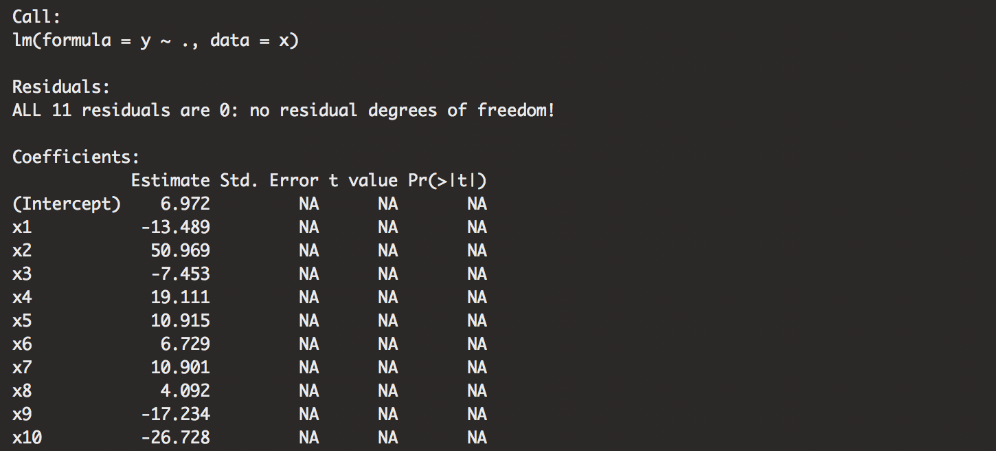
Remember, number of columns is p+1. Some call it k. We notice that we just have perfect fit models if the rows don’t exceed the columns.
AIC on the other hand is also a helpful object. AIC is (Akaike’s Information Criterion). It tries to answer, how much information is in the dataset that you can actually model? The formula is below.
## 2[-ln(L(est model)) + p*]
L(estimated model) stands for the Likelihood. In frequentist statistics, it is a parameter value “between 0:1” that maximizes the probability that we observe that value. Kind of tricky, so you might want to read up on it more. Since we’re not worried about the Bayesian case, it IS NOT a probability distribution of the parameter. Just another side-note.
p* stands for the # of estimated parameters (penalty. If you fit an overly complicated model). If the likelihood is big, the negative log likelihood is small, so “good” is “minimized”. Just note that the lower AIC is the best for prediction.
On the other hand, some people actually prefer to use the (BIC) Bayes information criteria (Actually, there is nothing remotely Bayesian about this value). This one is neat because if we take a look at the model, the bigger the p* doesn’t do much to correct adding too many variables. We know that adding more variables helps with R^2 interpretability, which is obvious, but we want to be putting more meaningful values (I guess that’s why the adjusted R^2 exists). The BIC converges to the true model if n goes to infinity, filling up data where we don’t have orthogonal information. In other words, BIC penalizes you for adding more values, but it depends on how many rows you have!
## 2[-ln(Likelihood(est model)) + p*ln(n)]
For the sake of interpretation, let’s just look at AIC. We’ll go into the data and start our model selection.
Data originally came from the NIH BioLINCC portal. You have to make an account to request the data and it takes about a day to receive it. Kind of a hassle to get approved. I also found other github libraries with the information, but I cleaned it for my purposes. You can take download mine from here. The data looks for patients that had or didn’t have any cardiovascular disease. I’m not much of a bioinformatics guy, but this is a neat dataset to work on our stepwise case! Just know that any analysis I make regarding health practices is definitely not informed. Just observed from the data!
Let’s get started. Our packages of interest are below. I won’t be explaining any of them, but the first one is a cleaning package, and ROCR is used for prediction performance concerning a Logistic Regression. I will hopefully be making a post about a logistic regression soon, but it might be a little while. It just takes a while to find fun data to work with and explain!
library(tidyverse)
library(ROCR)
Alright, first pull my data from the project page on my github repostitory.
url <- "https://raw.githubusercontent.com/tykiww/projectpage/master/datasets/Model%20Selection/frmgham2.csv"
t <- read.csv(url, header = T)
The data is subsetted to only participants that didn’t have Coronary heart disease. Afterwards, it was reduced to the risk factors we were interested in.
c("gender","cholesterol","age","BP","DBP","smoking","cigperday","BMI",
  "diabetes","BPmeds","heartrate","glucose","education","CVD")
You can disregard my organization of the data below. Just don’t forget to relevel the important factors of interest! I decided to change them to new values using an ifelse statement. for loops work just as well!
# subset to participants that didn’t have CHD
t <- t %>% subset(PERIOD==1 & PREVCHD==0)
# subset to risk factors under study
t <- t[,c(2:14,30)]
# Data check
head(t)[,1:5]
# Clean missing values
heart <- t %>% drop_na()
# check
dim(heart)
dim(t)
glimpse(heart)

# Change names
names(heart) <- c("gender","cholesterol","age","BP","DBP","smoking","cigperday","BMI",
            "diabetes","BPmeds","heartrate","glucose","education","CVD")

#make the variables interpretable
heart$gender <- ifelse(heart$gender==1,"m","f")
heart$smoking <- ifelse(heart$smoking==1,"smoker","nonsmoker")
heart$diabetes <- ifelse(heart$diabetes==1,"diabetic","nondiabetic")
heart$BPmeds <- ifelse(heart$BPmeds==1,"meds","nomeds")
heart$education <- ifelse(heart$education==1,"<HS",ifelse(heart$education==2,"HS",
                                                 ifelse(heart$education==3,"somecollege","college")))
Also one more thing to emphasize is to NOT change the predictor variable from 0,1 to yes, no or anything of that sort. For the logistic regression case, it makes it difficult to interpret in the future.
# Change to reasonable Factors
cols <- c("gender","smoking","diabetes","BPmeds","education")
heart[cols] <- heart[cols] %>% lapply(as.factor)
glimpse(heart)
lapply(heart[cols],levels) # checking levels
# releveling reference points
heart$gender <- relevel(heart$gender,ref="f")
heart$smoking <- relevel(heart$smoking,ref="nonsmoker")
heart$diabetes <- relevel(heart$diabetes,ref="nondiabetic")
heart$BPmeds <- relevel(heart$BPmeds,ref="nomeds")
heart$education <- relevel(heart$education,ref="college")
lapply(heart[cols],levels) # checking levels

Now, one of the key details not to miss is to create both train and test datasets. For prediction, we want to make sure that our values will extend to other situations. Remember to keep about 70-80% of the data in the training set and start working.
# Create Train and Test Datasets
set.seed(15)
round(dim(heart)[1]*.80) # 2926
train.ind <- sample(length(heart[,1]),2900)
h.train <- heart[train.ind,]
h.test <- heart[-train.ind,]

# remove vars
rm(t,cols,url,train.ind)
Here’s our data! Now, we’re able to look straight at finding the best predicting logistic regression model. Let’s look for the best means subset of all possible explanatory variables.
Here’s the forward selection case. I just named the variables “minmodel”, and “biggestmodel” just for interpretation sake. It’s pretty wordy, so probably not a good idea to do what I did here. Below are the forwards and backwards selection models. Don’t worry too much about these. Just know that these combined comprise the stepwise model.
# forward selection
minmodel.forward <- glm(CVD~+1,data=h.train, family="binomial")
biggestmodel.forward <- formula(glm(CVD~.,data=h.train, family = "binomial"))
out.framforward <- step(minmodel.forward,direction="forward",scope=biggestmodel.forward)

I’ve done a lot of explaining earlier, so I won’t write much here. Just know that the forward case starts with the minimum model, with no variables and builds the model until they have a model that creates the lowest AIC values.
# backawrds selection
out.frambackward <- step(glm(CVD~.,data=h.train,family="binomial"))

The backwards selection takes the whole model by specifying ~ . and works backwards by taking out the worst variables. Remember, we cannot do a backwards selection if number of columns don’t exceed the number of rows!
Now here’s the stepwise regression model! You can see how we specify “both” in the direction and the scope is the biggest model just as we created in the forward selection. Another note here, the order of the AIC values change, but the overall AIC, BIC, and adjusted R^2 values are not different accross all the models. If you decide that you want a smaller or bigger model, make sure to specify step = x inside of your step() function if you want a tune your model the way you like it.
# stepwise!
minmodel.stepwise<-glm(CVD~+1,data=h.train, family="binomial")
biggestmodel.stepwise<-formula(glm(CVD~.,data=h.train, family = "binomial"))
out.framstepwise<-step(minmodel.stepwise,direction="both", scope=biggestmodel.stepwise)

The output is large, so I will spare you the information besides the most important details. Our stepwise regression pulled out the most important variables. Our seemingly “best” model is shown as:
## CVD ~ BP + gender + age + diabetes + cholesterol + BMI + smoking + heartrate + DBP + education
Peculiar how the first variable it dropped was cigperday. It doesn’t mean that it is the least important. Probably, it just means that the AIC value wasn’t the best. Dropped probably because of some confounding with CURSMOKE. We can investigate further for other details.
summary(out.framstepwise)
##  Coefficients:
##                       Estimate Std. Error z value Pr(>|z|)
## (Intercept)          -8.873211   0.612167 -14.495  < 2e-16 ***
## BP                    0.011624   0.003535   3.288 0.001007 **
## genderm               0.830492   0.100556   8.259  < 2e-16 ***
## age                   0.048027   0.006383   7.524 5.32e-14 ***
## diabetesdiabetic      1.314523   0.257204   5.111 3.21e-07 ***
## cholesterol           0.005168   0.001081   4.783 1.73e-06 ***
## BMI                   0.042931   0.012364   3.472 0.000516 ***
## smokingsmoker         0.393556   0.100967   3.898 9.70e-05 ***
## heartrate            -0.010569   0.004106  -2.574 0.010049 *
## DBP                   0.015629   0.006442   2.426 0.015255 *
## education<HS          0.207222   0.162364   1.276 0.201856
## educationHS           0.369810   0.169600   2.180 0.029221 *
## educationsomecollege  0.025394   0.192757   0.132 0.895188
There may be things that aren’t statistically significant, but we used AIC to select the model. We are not trying to declare significance, but to predict well. So, if you see any insignificant values, don’t fret. It is a mid-way balance of interpretation and prediction. If you are looking for statistical significance, use SAS. SAS has a comparison of statistical significance with variable selection for prediction. R believes that in statistics, you shouldn’t really use statistical significance for best prediction.
Now another note, the most important factor is not the BP in the model. It just depends. Gender cannot be more important than diabetes, as it is something that cannot fix. For this case, let’s focus on things that can change. These come from the first question, not the first variable came in, but it is going to be what the doctors might ask first. “Where are you hurt?”, “What is your heartrate?”
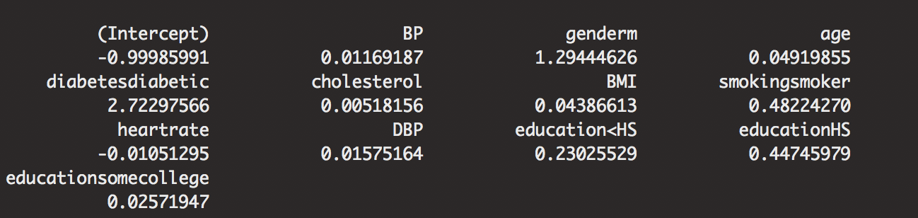
Of course, that does not mean we disregard the gender difference. We can estimate that men are 1.29 times more likely to develop CVD than women holding all other effects constant (95% CI: 0.8857, 1.7972). Other important effects, including this one is performed by taking the exponent of the log odds as shown below.
exp(coef(out.framstepwise))-1
exp(confint(out.framstepwise))-1
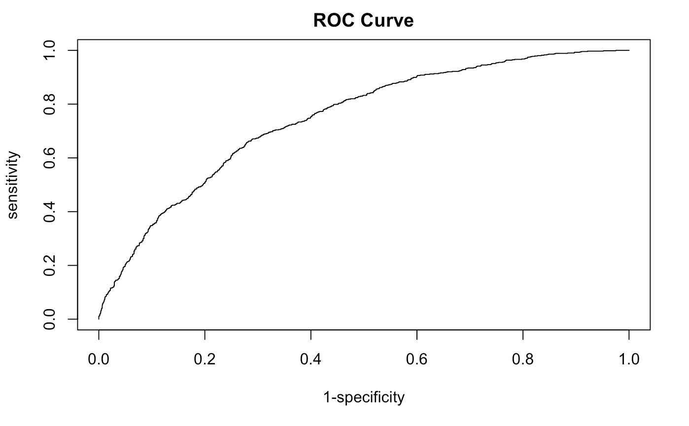
Instead of taking a look at more interpretations, constructing our ROC curve will help us see how our model prediction is doing for us. Our AUC value is 0.7461639, not bad, but not great. We see how the curve does not cover all of our interpreted values.
train.pred <- prediction(predict(out.framstepwise,type="response"),h.train$CVD)
train.perf <- performance(train.pred,measure="tpr", x.measure = "fpr")
plot(train.perf,xlab = "1-specificity",ylab = "sensitivity", main = "ROC Curve")
# AUC TRAIN
performance(train.pred,measure="auc") # 0.7461639
We’ll now compare both the Train and test AUC and plots together. Make sure to specify add=TRUE to lay one plot over the other.
# Test data
test.pred <- prediction(predict(out.framstepwise,newdata=h.test,type="response"),h.test$CVD)
test.perf <- performance(test.pred,measure="tpr", x.measure = "fpr")
plot(test.perf,xlab = "1-specificity",ylab = "sensitivity",
     main = "ROC Curve", add= TRUE, col = "royalblue")
# AUC TEST
performance(test.pred,measure="auc") # 0.7285064 pretty good but not great.
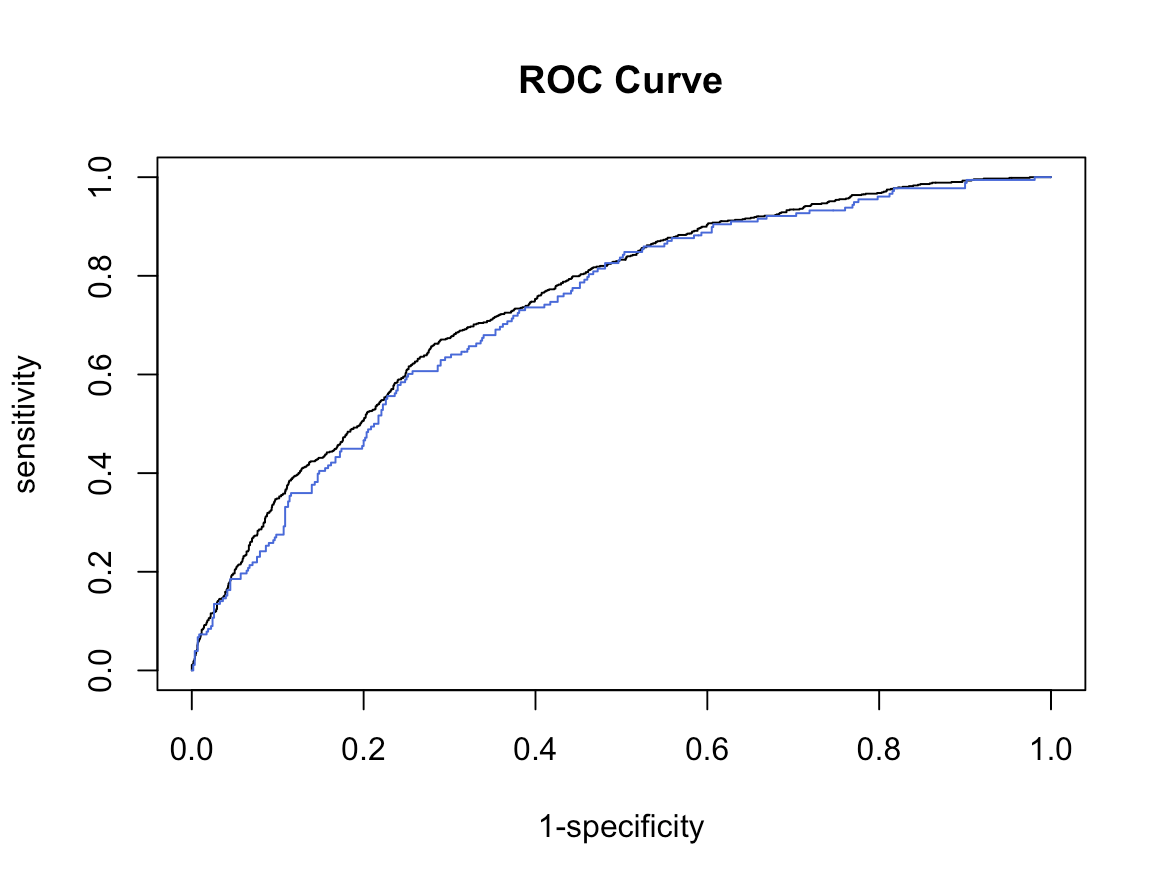
Not bad, our test case does not predict as great as our training data. This isn’t a bad thing since it’s so close. Just know that there is variation when we are trying to predict out of this example!
Overall, I have some important thoughts to note.
Statistical significance was not key to choosing our model. I guess this is more important if you are focused on a more regression (interpretation) model. Of course, this is a regression model, but we just realize, with such a big dataset that even these values seem to influence in some ways. We probably need more data to interpret.
Sometimes these variables can come up with the wrong sign. If so, we can always check for collinearity and/or look for the next best variable that comes up. Unfortunately for our case, the information just isn’t interpretable.
Also, good to note that hypothesis test results don’t need to be reported. Neither are they fair. If we’re not using that to predict some values that aren’t significant, we should probably be wary about including these values in our future model.
Don’t forget! Just because something is omitted, doesn’t mean it is important. This is where we need to be careful with our supervised machine learning case. When we have so much information, our data will hopefully converge to the distribution that the world follows.
I’ll hopefully be working on a post about Lasso regression technique sometime! The lasso case will allow us to find any latent casess of explanatory variables. These Big Data techniques are in demand and become extremely useful, so hopefully this will come in handy for you!