Let’s say you own a bike-sharing company and you’ve gathered a whole bunch of data that you don’t know what to do with. Your main goal is to be able to predict how many riders you will have at any given point of the day. Using this information, we are hoping to establish full-time equivalent benchmarks of good and bad performance.

While this problem may be easily solved with any type of regression, we will be hoping to improve our performance using an ensemble weighted-average approach.
Ensemble Weighted AVerage
Like any ensemble method, the whole goal is to combine multiple models to solve the same problem in hopes of improving our results. The hope is to combine these weak models to obtain more robust estimates.
Many times, we are faced with the bias-variance problem. This problem is a tradeoff of models having either too high of a bias (e.g. having low numbers/quality of independent factors or bad model assumptions) OR high variance (i.e. model is too sensitive to noise and specifics of the data).
Most of the time, high bias in an algorithm means less variance, and vice versa.
The weighted average, along with many other ensembles, seeks to mitigate this issue. It takes the average of all predictions and weights them probabilistically on how trustworthy they are. By taking a combinatorial approach of low variance and low bias models, the tradeoff becomes limited to be both high-perfoming and robust. You’ll notice here that when I say performance, it doesn’t neccesarily mean to completely minimize the error between the predictions and the dependent variable. In many cases, this weighted average will improve performance when combining lots of weak predicting models. However, when we decide to use weak and strong performers, this can be a conservative approach against overfitting.
Bike-Sharing Case
Our north-star metric is the total number of riders. Therefore, our goal is to benchmark what is typical day to day given a variety of outputs. If we happen to go above our predicted outputs, we know that we are going above the typical performance.
Let’s say in our database we have the following data:
library(tidyverse, quietly = TRUE)
url <- "https://raw.githubusercontent.com/tykiww/projectpage/master/datasets/BikeShare/bike%20data.csv"
dtset <- read_csv(url)

# Split Dates
dtset <- separate(dtset,"Date",c("Day","Month","Year"),"/")
dtset[,c(1:3)] <- apply(dtset[,c(1:3)],2,as.numeric)

# Remove Casual and Registered Users
dtset <- dtset[,-c(3,14:15)]

# Change Names
cols <- c("Day","Month","Season", "Hour", "Holiday","Day_of_Week", "Work_Day","Weather","Temp",
          "Temp_Feels","Humidity","Wind_Speed","Total_Users")
colnames(dtset) <- cols

# Split Train/Test
idd <- sample(1:nrow(dtset),.8*nrow(dtset), replace = FALSE)
train <- dtset[idd,]
tests <- dtset[-idd,]

# Quick Skim
skimr::skim(dtset)
## Skim summary statistics
##  n obs: 17379
##  n variables: 13
##
## -- Variable type:numeric -------------------------------------------------------
##     variable missing complete     n    mean     sd   p0  p25   p50   p75  p100     hist
##          Day       0    17379 17379   6.54    3.44  1    4     7    10    12   ▇▅▇▃▅▇▃▇
##  Day_of_Week       0    17379 17379   3       2.01  0    1     3     5     6   ▇▇▇▇▁▇▇▇
##      Holiday       0    17379 17379   0.029   0.17  0    0     0     0     1   ▇▁▁▁▁▁▁▁
##         Hour       0    17379 17379  11.55    6.91  0    6    12    18    23   ▇▇▇▇▇▇▇▇
##     Humidity       0    17379 17379  62.72   19.29  0   48    63    78   100   ▁▁▃▇▇▇▇▅
##        Month       0    17379 17379  15.68    8.79  1    8    16    23    31   ▇▇▇▇▆▇▇▇
##       Season       0    17379 17379   2.49    1.12  1    1     2     3     4   ▇▁▇▁▁▇▁▇
##         Temp       0    17379 17379  58.78   16.62 17.6 45.2  59    72.8 102.2 ▁▅▇▇▇▇▃▁
##   Temp_Feels       0    17379 17379  59.72   20.42  3.2 42.8  60.8  77   122   ▁▃▆▇▇▆▁▁
##  Total_Users       0    17379 17379 189.46  181.39  1   40   142   281   977   ▇▅▂▂▁▁▁▁
##      Weather       0    17379 17379   1.43    0.64  1    1     1     2     4   ▇▁▃▁▁▁▁▁
##   Wind_Speed       0    17379 17379  12.74    8.2   0    7    13    17    57   ▇▇▇▂▁▁▁▁
##     Work_Day       0    17379 17379   0.68    0.47  0    0     1     1     1   ▃▁▁▁▁▁▁▇
Now, we can see some interesting summary statistics here such as individuals tend to bike share less during holidays/weekends and more during weekdays. Useage reports higher values during a “middle” temperature value These items indicate a seasonality that will be hard for a regular regression to detect.
Ensembling!
Let’s begin first by ensembling a few learners. Three models in particular seem to fit the bill: Random Forest, Recursive Partitioning, and XGBoost. The reason these may perform better than OLS or GLM regressions is because of the seasonality we noticed earlier. Bagging and decision trees seem to be a better option for performance. We will not be doing any parameter tuning for these models. Technically, we are ensembling some ensemble models, so hopefully we will still see some good performance gains.
library(randomForest, quietly = TRUE)
library(rpart, quietly = TRUE)
library(xgboost,quietly = TRUE)

# RF, Recpart, and XGB
m1 <- randomForest(Total_Users ~., data = train)
m2 <- rpart(Total_Users ~., data = train)
dtrain <- xgb.DMatrix(data = as.matrix(train), label = train$Total_Users)
dtests <- xgb.DMatrix(data = as.matrix(tests), label = tests$Total_Users)
m3 <- xgboost(data = dtrain,label = train$Total_Users,max.depth = 2, eta = 1, nthread = 2, nrounds = 2)
Instead of going into the summaries, we will just proceed to predict using both training and test data. If we are hoping for interval estimates, we should specify in our predictions predict.all=TRUE or some interval= statement.
# Create Training Predictions
p1 <- predict(m1, newdata = train)
p2 <- predict(m2, newdata = train)
p3 <- predict(m3,dtrain)

# Create Testing Predictions
pp1 <- predict(m1, newdata = tests)
pp2 <- predict(m2, newdata = tests)
pp3 <- predict(m3,dtests)
Now our predictions are complete! It is time to do our weighing.
Weights can be done in various ways. However, probably the most useful is using a random forest or a regression.The steps here are simple. 1) Create a dataframe of each predictor as an X matrix. 2) The y vector for our regression output will be the original dependent variable from our testing set. 3) Calculate the absolute effect of each model on the dependent variable and weigh them from out of the sum effect USING THE TEST DATA 4) Multiply the probabilities with each prediction.
Another approach to finding the best probability ratios is by just gridsearching our way to the best estimate. However, what’s the fun of brute-forcing our way into everything when we can finesse with real analytics? Isn’t that the point of learning this stuff? Note here, however that brute force gridsearch may come up with a more accurate estimate. Yet, these are estimates and are only as reliable as the method we use.
# Creating X and y matrix (rf and regression takes care of intercept
dtests <- data.frame(outs = tests$Total_Users ,cbind(pp1,pp2,pp3))
rownames(dtrain) <- NULL

# Perform Regression this time.
ob_tests <- lm(outs ~.,data = dtests)

relative_coeffs <- sapply(1:3,function(i)ob_tests$coefficients[-1][i]*median(dtrain[-1,i]))
(prbs <- abs(relative_coeffs)/sum(abs(relative_coeffs)))

# Multiply with prediction
trainpred <- sapply(1:3, function(x) prbs[x]*get(paste("p",x, sep = ""))) %>% rowSums()
testspred <- sapply(1:3, function(x) prbs[x]*get(paste("pp",x, sep = ""))) %>% rowSums()

# Compare with Straight Average
nowttrain <- (p1+p2+p3)/3
nowttests <- (pp1+pp2+pp3)/3
    ##        pp1        pp2        pp3
    ## 0.31034146 0.02346618 0.66619236
Using our testing data to generate probabilities, XG Boost seems to be our number one model with Random Forest and decision trees falling further behind. The reason why we use the test data to generate our predictions rather than the training data is because everything we do moving forward in prediction is based on unseen samples. If we use the probabilities of the training data, we will risk overfitting even more to our original model outputs.
rmse <- function(yi,yhat) sqrt(mean((yi - yhat)^2))

# Training Prediction rmse
tr <- cbind(Combined = rmse(trainpred, train$Total_Users),
            Straight = rmse(nowttrain, train$Total_Users),
            rbind(sapply(1:3, function(x) rmse(get(paste("p",x, sep = "")),train$Total_Users))))
colnames(tr) <- c("Combined", "Straight","p1","p2","p3")
ts <- cbind(Combined = rmse(testspred, tests$Total_Users),
            Straight = rmse(nowttests, tests$Total_Users),
            rbind(sapply(1:3, function(x) rmse(get(paste("pp",x, sep = "")),tests$Total_Users))))
colnames(ts) <- c("Combined", "Straight","p1","p2","p3")
c1 <- rbind(tr,ts); rownames(c1) <- c("Train","Test")
c1
    ##       Combined Straight       p1       p2       p3
    ## Train  32.5351 46.05146 33.40411 104.1434 45.24019
    ## Test   37.5655 54.97742 65.57628 103.7834 45.13202
Here we see the prediction RMSE outputs. Immediately, we notice here that our combined model has the best RMSE and performs better than every single grouping. Random Forest seems to be completely overfitting whereas the other models are very consistent accross the board. Although our RF has been overfitting, the Combined Train-Test estimate is not overfit due to the offset of the other models. By weighting our predictions, we were able to mitigate our high variance issue that came from the random Forest while also increasing RMSE overall. It really is the best of all worlds.
Interpreting output
Simply here, our output is our previous performance benchmark. The goal is to exceed what is predicted for the future. If we gain riders below this prediction, we are underperforming in this time frame. If we obtain riders above this prediction, we are performing above what we predict to expect.
train <- as_tibble(cbind(train,"Predicted"= trainpred))
tests <- as_tibble(cbind(tests,"Predicted"= testspred))
tail(tests)[10:14]
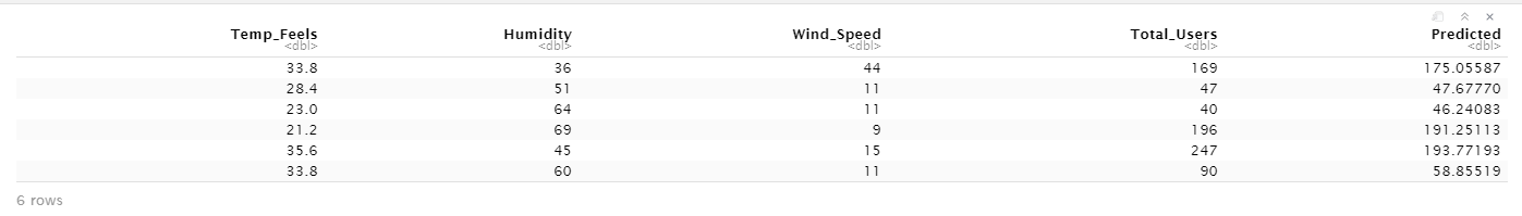
I just chose the tail test estimates just so you can see how close we can get with our estimates. We aren’t spot on, but we are close.
total <- rbind(train,tests)
mean((total$Predicted-total$Total_Users) > 0)
# [1] 0.541343
On average, we are going to be overestimating our predictions by 54%. This, for our case is a great thing because this can encourage our employees to expect a higher standard. We noticed previously that our RMSE is in between 32-37 which indicates a higher possible gap on average.
Remember, these are benchmarks against past performance!! This means it can technically be treated like the real Total Users value.
Other Notes
Hopefully this opens your eyes on the power of ensemble models and how you can go on to build one yourself. We did not cover categorical estimates, but you can see how changing the weighting model type from regression to classification (multinomial, logistic, rf) can yield the desired estimates. Furthermore, it is important to note that performance gains are realized when the model itself uses independent data. Scrambling image, sound, table data into three separate models and averaging can potentially impact your performance by quite a margin. Good luck on your next project!