Intuition vs. Pure Data (with a ton of assumptions..)
I have posted a few basic bayesian analysis techniques that are simple in terms of code. I even have a whole analytical collection if you’re curious of anything past the basics. However, I have never written a detailed explanation for why a Bayesian method differs so much compared to the traditional frequentist method. It’s quite simple. However, it really isn’t trivial. We will be doing a shallow dig into why Bayes trumps Frequentists (not being partisan here at all..).

Really, there are so many reasons why the Frequentist method is just ‘not as great’. Let’s just take a few of these and dissect them one at a time.
1) Sampling Distributions… 2) Rejecting the null?? 3) Parameters are fixed and unknown 4) The issues with unequal variance 5) Frequentists think bias is bad
(1) Sampling Distributions
If we take apart the classical t-test (t.test) we get something that looks like this.
t_test <- function(x,mu = 0, alpha = .05) {
  # Prerequisite
  xbar <- mean(x)
  vbar <- var(x)
  n <- length(x)

  # Calculate t-statistic, p-value, and confidence interval
  t_stat <- (xbar - mu) / sqrt(vbar / n)
  p_val <- 2 * pt(-abs(t_stat), n-1)
	conf_int <- xbar + c(-1, 0, 1) * qt(1 - alpha / 2,df= n-1) * sqrt(vbar / n)

	# Return Results
	output <- list("T-Statistic" = round(t_stat, 3),
	               "P-value" = round(p_val, 3),
	               "Confidence Interval with Mean" = round(conf_int, 3))
	return(output)
}
$\overline{x}$ is assumed to be distributed normal. In hand-wavy terms, this means that the probability of finding the true estimate (mean, $\overline{x}$) follows a gaussian (normal) character.
This theory is based on the sampling distribution. The notion is that if we drew more and more samples, they will each have a different mean (that’s not wrong). IF the distribution of x itself is normal, then the distribution of $\overline{x}$ should also be normal . Therefore, the average of the sampling distribution should approximate to the ‘True’ mean value (Central Limit Theorem) IF sampled over and over again. This allows for us finding the “true” fixed estimate of x and can be expressed in the form of a confidence interval estimate.
But wait! How sure are you that the mean is actually in the interval even if we sampled over and over again? “We are 95% confident..” Actually, we don’t know whether the mean is in or not in the interval (it’s really not useful information). We are ‘confident’ in the method that 95% of the time the interval will contain the true paramete IF we repeated this sampling process n number of times….
Well duh. That’s like saying if I took the average of all the samples of almost the whole population, I should get the true mean. We know linearity of expectation (taking the average of an average is still the average) holds, but the confidence interval doesn’t really tell us anything because we actually HAVEN’T sampled the procedure more than once. As a bayesian, you have no need to use a sampling distribution. An estimate comes from within a probability distribution which is a whole other thing. If you are frequentist, you have no framework to do a problem without a sampling distribution.
(2) Rejecting the Null
What is the null really? The confidence interval is already an implicit hypothesis test, so we already know that there are potential faults. You cannot do frequentist work without a null space. There needs to be some constraint. 90% confidence? 80% confidence? On what basis should we decide? What happens when a parameter can be both null and not at the same time? (That’ll come next). For Bayesians, it’s simple, p-values are useless. The bayesian paradigm (hand-waving here) mimicks the law of probability (with a lot of measure theory backing it up).
\[Posterior(parameters|data) \propto Likelihood(data|parameters)*Prior(parameters)\]Don’t get me wrong. I do think hypothesis testing is a really important logical tool for inference. But it works best if parameters are fixed.
(3) Paremeters are fixed and unknown
What I mean by parameters being fixed and unkown is this: Any estimate (mu, sigma) is UNCHANGING and can never really be known.
Are all parameters fixed and unknown? Not always; for the most case, paramters are always changing. Let’s take for example sports. Am I to believe that Lebron James’ skills have a true fixed level?
Bayesians will say otherwise: Any estimate (mu, sigma, etc) is frequently changing and CAN be known by a probability distribution.
# Lebron Field Goal Average (All teams)
fga <- rev(c(19.9,19.3,18.2,18.6,18.5,17.6,17.8,18.9,18.8,20.1,19.9,21.9,20.8,23.1,21.1,18.9))
x <- seq(length(fga))+2003
qplot(x, fga, geom = 'line', xlab = "Year", ylab = "Field Goal Average")
# Data from https://stats.nba.com/player/2544/
We can say prior to our estimation, that Lebron has a certain estimate right now. As we use the data and assume that his success follows a fitting distribution, we can model an unchanging estimate that fits a proper distribution.
The Bayesian method of updating prior distributions using the data (likelihood) into current posteior and predictive distributions is very intuitive. Your thoughts + data = new thoughts. It really pays off to have parameters as probability densities (think of a Bayesian parameter as a random variable) especially when you can make intuitive assumptions.
(4) Issues with unequal variance
What if you had data that looks like this.
library(skimr)
values <- c(121,94,119,122,142,168,116,172,155,107,180,119,157,101,145,148,120,147,125,126,125,130,130,122,118,118,111,123,126,127,111,112,121)
groups <- c(1,1,1,1,1,1,1,1,1,1,1,1,1,1,1,1,1,1,1,2,2,2,2,2,2,2,2,2,2,2,2,2,2)
two_groups <- data.frame(values,groups)
skim(two_groups)
## Skim summary statistics
##  n obs: 33
##  n variables: 2
##
## -- Variable type:numeric -------------------------------------------------------
##  variable missing complete  n   mean    sd p0 p25 p50 p75 p100     hist
##    groups       0       33 33   1.42  0.5   1   1   1   2    2 ▇▁▁▁▁▁▁▆
##    values       0       33 33 129.03 20.14 94 118 123 142  180 ▁▂▇▂▂▂▁▁

## variance [group 1]    791.0
## variance [group 2]     62.6 # Whoa, can't do much frequentist stuff with that kind of difference in variance.
Can you really perform a two-sample t-test? Or for that matter, any statistical test? In any test: When your assumptions break, your models break. But wait, how about Welch’s two-sample t-test with unequal variances? Yeah, that could work? But there is no closed form (cannot be evaluated in a finite number of standard operations). Plus, how are we going to decide the degrees of freedom analytically???
Bayes can take care of that unequal variance by just “integrating” out the variance (Just a fancy way of telling the computer to toss it out. Or you can do the math if it has a closed form, bleh).
## P(A n B) = P(A)P(B) iff A & B are independent
## p(A n B) = p(A|B)P(B) = P(B|A)P(A)
## p(A|B) = p(B|A)P(A)/P(B) # integrate out A space to get B space (integrate out the parameters to get the data).
library(rjags)
library(R2jags)


# two sample t-test. Do they have the same means?


# 33 datapoints
# 2 is for each treatment

mdl <- "
model {
  for (i in 1:33) {
  y[i] ~ dnorm(mu[tmt[i]], 1/vr[tmt[i]])
  }
  for (i in 1:2) {
    # Unknown Mean (assumed normal, HIGH variance/low precision)
    mu[i] ~ dnorm(0,0.000001)
    # Unknown Variance (uninformed)
    vr[i] ~ dunif(0,5000)
  }
}"

# Save Model
writeLines(mdl,'twogroups.txt')

# Specify parameters for model
tmt <- two_groups$groups
y <- two_groups$values
data.jags <- c('tmt','y')
parms <- c('mu','vr')

# Run Model
twogroups.sim <- jags(data= data.jags, inits = NULL, parameters.to.save=parms,
                      model.file='twogroups.txt', n.iter=50000, n.burnin=10000,
                      n.chains = 5, n.thin = 5)

# Grab the outputs

sims <- as.mcmc(twogroups.sim) # Coerce simulation as mcmc object
chains <- as.matrix(sims) # Grab the matrixed chains


# IS GROUP 1 larger than Group 2?

sprintf("The posterior probability that group 1 is bigger than group 2 is %s", mean((chains[,2] - chains[,3]) > 0))
## [1] "The posterior probability that group 1 is bigger than group 2 is 0.973125"
Yes, that was a LOT more work than just running t.test(). However, we have reliable estimates. And I mean REALLY realiable. No worries about the variance and no need for a p-value. How much greater can it get?
(5) Frequentists think Bias is bad
Honestly, this is a flawed argument (I’ve probably been making a ton of those in this post). What is not unbiased about a degree of freedom? Technically, an assumption is a bias as well. As you get more complicated with frequentist work, most things are biased. You just can’t escape it. Plus, what’s wrong with bias anyways?
If you knew that an UNBIASED coin (p = .5) was flipped once and you landed tails. If you were a frequentist, what would you say the true probability is?
data <- c(0)
t.test(data)
## Error in t.test.default(data) : not enough 'x' observations
Can’t do it! Error..
How about if you landed tails 5 times in a row?
data <- c(0,0,0,0,0,0)
t.test(data)
##  	One Sample t-test
##
##  data:  data
##  t = NaN, df = 6, p-value = NA
##  alternative hypothesis: true mean is not equal to 0
##  95 percent confidence interval:
##   NaN NaN
##  sample estimates:
##  mean of x
##          0
What do you even learn from this? That the true probability of getting a heads is 0? We know that we’ll get a heads somewhere and it’ll probably even out (law of large numbers).
If you have experience or strong intuition and data is sparse, wouldn’t you favor that experience?
# Farily confident that out of 10 samples, 5 will be heads.
# Expectation: 0.5 = a/(a+b)
# prior
a <- 5
b <- 5
k <- sum(data)
n <- length(data)
# posterior is a + K; n - k + b
post_a <- a + k
post_b <- n - k + b
# Our new "middle" estimate
sprintf("%s posterior probability that the parameter is heads",qbeta(.5,post_a,post_b))
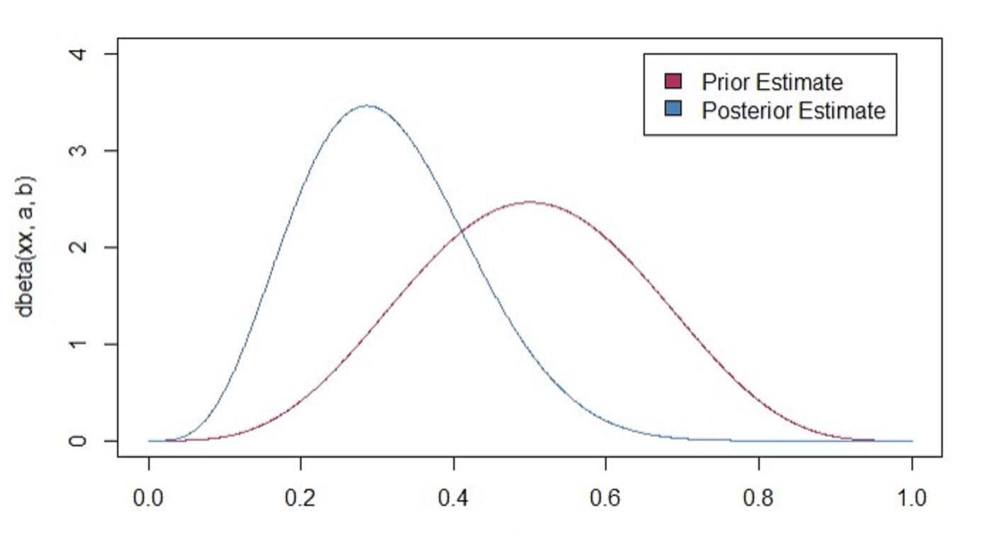
xx <- seq(0,1,length.out = 1001)
plot(xx,dbeta(xx,a,b), type = "l", col = "maroon", xlim = c(0,1), ylim = c(0,4))
lines(xx,dbeta(xx,post_a,post_b), col = "steel blue")
legend(.65,4,c("Prior Estimate", "Posterior Estimate"), c("maroon","steel blue"))
## [1] "0.304519809633879 posterior probability that the parameter is heads"
Even with limited data, we are still able to inference because of our previous distributional assumptions or our bias. Maybe it is more biased than we think! Even thought I don’t know where the estimate is, I can make some sort of intuition using distribution by narrowing where I am looking for. Now, the more data we have, the closer we get to our frequentist estimates. In this data-rich age, you won’t go wrong using either methods when assumptions don’t break. However, keep in mind that not all decisions made are done through big data! Most of the time, we are pitted against making a decision with no information at all! Bayesian techniques are most powerful when making strategic decisions with limited data .
Conclusion
Now, this post is definitely biased, and I am okay with that. It really is up to you on how you view the world. I still mostly use frequentist methods because it is faster and can be easier. Plus, I am not smart enough to just create my own bayesian techniques all the time. However, I feel that I am a more intuitive individual and this really speaks to me in terms of decision making. If our assumptions were wrong, we are wrong. At least we didn’t just sit around and say we can’t do anything about it.