Recently, in my world, data storage and computation has been a normal issue. Even with alloted space, I had seemingly reached across the limits set for my schema without drawing a single breath. As an analytics practitioner, this is always a concern. On the other hand, storage is cheap, really cheap; why shouldn’t we buy or request more? However, it is like knowing your surroundings. Understanding the data goes further than just knowing what to calculate with limited amounts of it. Each byte counts and if you’re not aware of how much every data point costs it could potentially byte you in the butt.

In this post I have broken down simple ways to determine how you can scale your data before you start dumping large amounts of it. Each type of data really all comes down to bytes. How many bytes?

• tables:

Tables can get complicated. Each datatype yields different results, so the relationship can become multivariate linear. A 1 by 1 dataframe of characters is ~60% larger than a 1 by 1 dataframe of numeric variables. Say you had a 100 by 100 table which had 20 columns of characters. How big would that be?

cost_calculation<- function(nbyn = 100,mixp = .8) {
  
  ob <- sample(c(TRUE,FALSE),size = 1,
               prob = c(mixp,1-mixp), 
               replace= TRUE)
  
  ic <- matrix(NA,nrow=nbyn,ncol=nbyn)
  n <- 0
  for (i in 1:nbyn) {
    for (j in 1:nbyn) {
      n <- n + 1
      m <- matrix(ifelse(ob,1,"1"),nrow=i,ncol=j)
      m <- as.data.frame(m)
      ic[i,j] <- object.size(m)
    }
  }
  
  rownames(ic) <- 
    colnames(ic) <- 1:nbyn
  
  return(ic)
}
a <- cost_calculation(100,.8)
a[100,100]

[1] 92608

93 kilobytes. That barely makes a dent. However, if we were to plot each average increase in row or column, we see clear linear patterns of increase.

par(mfrow=c(1,2))
plot(1:99,
     diff(colMeans(a)), 
     type = 'l', col = "steel blue",
     ylab = "Average Byte Increase",
     main = "Column Difference",
     xlab = "")
plot(1:99,
     diff(rowMeans(a)), 
     type = 'l', col = "steel blue",
     ylab = "Average Byte Increase",
     main = "Row Difference",
     xlab = "")
title("Average Byte Increase for every Row/Column Increase",line = -21, outer = TRUE)
par(mfrow=c(1,1))

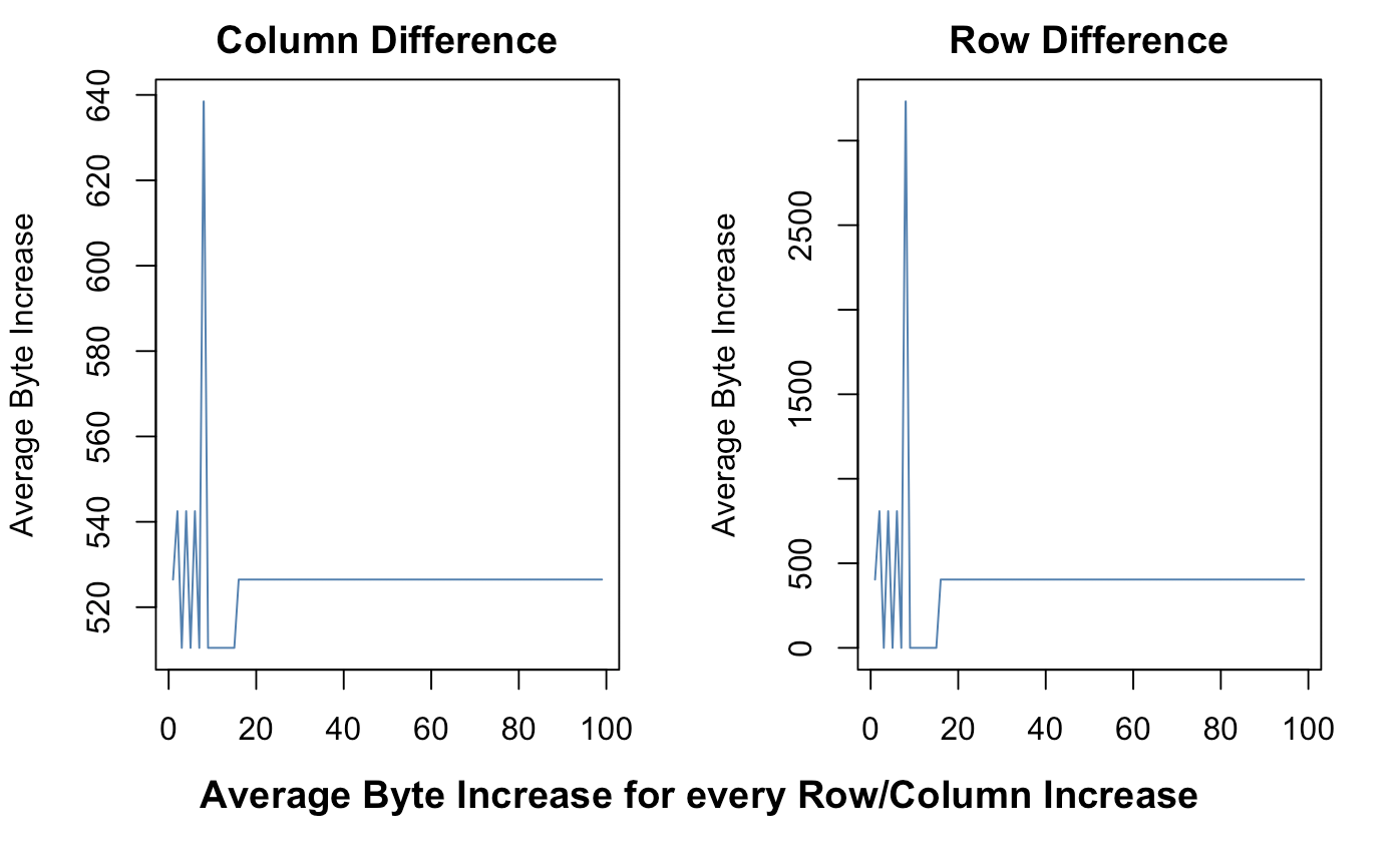
There is some volitility with smaller data, but as p and n increase the change ends up sharply linear. For each increase in column, the average increase of bytes, holding the count of rows constant, is an average of 525. For each row increase the average is under 500. When scaling each byte. This means that we can make a regression function to estimate how much data a particular table will use.

# y = m1x1 + m2x2 + b

howmuch <- function(nbyn, m1, m2, b) m1*nbyn + m2*nbyn + b

howmuch(100, mean(diff(colMeans(a))),
        mean(diff(rowMeans(a))), 736)

[1] 93784

Not bad of an estimate compared to our original 92,608 output.

• images & videos:

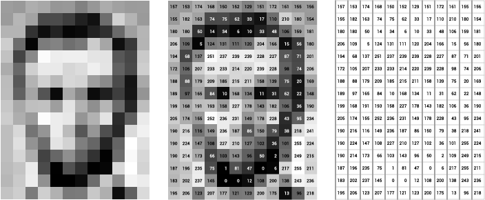
Images are a lot more straightforward. Take a particular shot of this car for example (640 x 478 x 3)

This means that our image is has a total of 640*478 = 305920 pixels. Luckily for us, pixels scale by a factor of 3 (rgb). So our total byte count is 640*478*3 = 917760 (almost as many bytes as that table above). If you have more images with a shape of (1000 x 640 x 478 x 3) you’ve already got 1 gigabyte of images.

On the other hand, videos are just stacks of images. So, the calculation is similar as above. Think about that next time you do any computer vision projects.

• sound:

Sound can be a bit more challenging to deal with. It really depends on the sampling frequency. When processing signals, sound waves are digitized as flat arrays sampled at discrete intervals. Typical samples are taken 44,100 or 65,536 times each second at each amplitude of a sound wave. These then can be converted to bits depending on how detailed the sample will be. Let’s take a look at how this plays out.

library(dplyr)
library(wrassp)
wvf <- system.file('extdata', package='wrassp') %>%
  list.files(., pattern=glob2rx('*.wav'), full.names=TRUE)
(play <- read.AsspDataObj(wvf[1]))

Assp Data Object of file /Library/Frameworks/R.framework/Versions/3.5/Resources/library/wrassp/extdata/lbo001.wav.
Format: WAVE (binary)
19983 records at 16000 Hz
Duration: 1.248938 s
Number of tracks: 1 
	 audio (1 fields)

attributes(play)

$names
[1] "audio"

$trackFormats
[1] "INT16"

$sampleRate
[1] 16000

$filePath
[1] "/Library/Frameworks/R.framework/Versions/3.5/Resources/library/wrassp/extdata/lbo001.wav"

$origFreq
[1] 0

$startTime
[1] 0

$startRecord
[1] 1

$endRecord
[1] 19983

$class
[1] "AsspDataObj"

$fileInfo
[1] 21  2

We have a very low sample rate (16000) audio file which only lasts about one second. Each integer is the amplitude of the collected sample.

head(c(play$audio))

[1]  5 -2 17 -5 -5 -2

Just for our sanity, if the sample rate was 16,000 then we should easily be able to decipher the sample length.

as.integer(16000*1.248938) # sample rate per second = total integer length

[1] 19983

Spot on! Now we’ll continue by deciphering how many bytes each integer holds.

paste('depth:',object.size(c(play$audio))/19983,'bytes per sample')

[1] "depth: 4.0026022118801 bytes per sample"

This means that each second holds about 4 bytes of information each. Now, just a disclaimer, this depends on the quality of the sound. Higher quality audio will have larger byte depths. With this information we can create a short formula.

In our case, if we had a 3 minute audio clip, we will have a total byte count of:

object.size(c(play$audio))/19983*180*16000

11527494.4 bytes

A total of 11.5 megabytes. So, the trick is.. Take a small sample, figure out the byte depth, then scale to the desired sample rate per second. Then, you’ll really know how much data you’re working with.

Of course, this isn’t the only form data can take. Coordinate data can be as simple as a table whereas GIS information will become inordinately heavy. However, the framework for figuring out space is the same for all types of data. Just condense things into manageable byte size chunks and scale up for prediction!