What parameters from an EEG scan are most critical to understanding whether the eye moves or not?
EEG is a shorthand for an Electroencephalogram. It is a brain-activity monitor. To be honest, I have no idea how it works but we have some data and parameters to guide our decisions. The data below was collected to monitor eye Detection. Can the parameters collected by the scanner detect if your eye is moving? In many ways, it is an evaluation of the EEG machine.
Now there are many ways to answer this question. We could visualize and see if there is a visual/linear trend. However, we have all these knobs that we can turn and understand. Using a logistic regression seems like a reasonable choice!
Logistic vs OLS?

Logistic Regression, the counterpart to OLS regression, is a powerful binary classification technique classically applied by many. Instead of looking to understand our y value on a continuous scale, we want to understand the probability of y occuring (1 for yes, 0 for no).
In an ordinary least squares regression, the equation looks like this
\[y = \beta_{o} + \beta_{n}x_{n} +\epsilon\]Now, what if we were looking for the probability that y = 1?
\[p(y=1|x) = \frac{e^{\beta_{o} + \beta_{n}x_{n} +\epsilon}}{1 + e^{\beta_{o} + \beta_{n}x_{n} +\epsilon}}\]Don’t get freaked out by the notation. This equation comes from assuming that our binary y comes from a sigmoid distribution. This ratio can be rearranged to look like our OLS regression if we create a log odds ratio.
\[log(\frac{p(y=1|x)}{1-p(y=1|x)}) = \beta_{o} + \beta_{n}x_{n} +\epsilon\]Odds are just an odd way to look at probabilities (direct shot at my British friends).
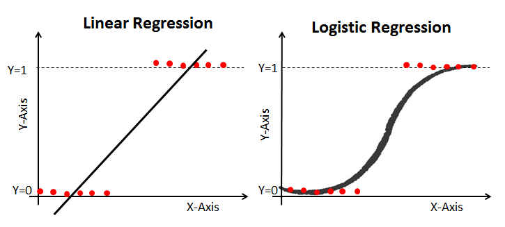
Image from datacamp.com.
The benefit of using the sigmoid distribution is three reasons. 1) The sigmoid is differentiable accross its entire range, 2) it is easy to compute, and 3) it is restricted between [0,1].
Now keep in mind that this will change regression coefficient interpretation and way we do predictions. We will get into that real soon.
There is more to a logistic regression (e.g. using maximum likelihood vs OLS to estimate parameters). However, we’ll just cover the most important bits and get along to analysis. I firmly believe that the interpretation of the method yields more positive benefits than going too deep into the mathematics. The math will catch up after you learn to interpret it.
Data Read In
Data comes from my repository and can be read in here.
library(tidyverse, verbose = FALSE)
url <- "https://raw.githubusercontent.com/tykiww/projectpage/master/datasets/EEG/EEGEyeState.csv"
eeg <- read_csv(url)
skimr::skim(eeg)
## Skim summary statistics
##  n obs: 14980
##  n variables: 15
##
## -- Variable type:numeric -------------------------------------------------------
##      variable missing complete     n    mean      sd      p0     p25     p50     p75      p100     hist
##           AF3       0    14980 14980 4321.92 2492.07 1030.77 4280.51 4294.36 4311.79 309231    ▇▁▁▁▁▁▁▁
##           AF4       0    14980 14980 4416.44 5891.29 1366.15 4342.05 4354.87 4372.82 715897    ▇▁▁▁▁▁▁▁
##  eyeDetection       0    14980 14980    0.45    0.5     0       0       0       1         1    ▇▁▁▁▁▁▁▆
##            F3       0    14980 14980 4264.02   44.43 1040    4250.26 4262.56 4270.77   6880.51 ▁▁▁▁▇▁▁▁
##            F4       0    14980 14980 4279.23   41.54 2257.95 4267.69 4276.92 4287.18   7002.56 ▁▁▁▇▁▁▁▁
##            F7       0    14980 14980 4009.77   45.94 2830.77 3990.77 4005.64 4023.08   7804.62 ▁▇▁▁▁▁▁▁
##            F8       0    14980 14980 4615.21 1208.37   86.67 4590.77 4603.08 4617.44 152308    ▇▁▁▁▁▁▁▁
##           FC5       0    14980 14980 4164.95 5216.4  2453.33 4108.21 4120.51 4132.31 642564    ▇▁▁▁▁▁▁▁
##           FC6       0    14980 14980 4202.46   37.79 3273.33 4190.26 4200.51 4211.28   6823.08 ▁▁▇▁▁▁▁▁
##            O1       0    14980 14980 4110.4  4600.93 2086.15 4057.95 4070.26 4083.59 567179    ▇▁▁▁▁▁▁▁
##            O2       0    14980 14980 4616.06   29.29 4567.18 4604.62 4613.33 4624.1    7264.1  ▇▁▁▁▁▁▁▁
##            P7       0    14980 14980 4644.02 2924.79 2768.21 4611.79 4617.95 4626.67 362564    ▇▁▁▁▁▁▁▁
##            P8       0    14980 14980 4218.83 2136.41 1357.95 4190.77 4199.49 4209.23 265641    ▇▁▁▁▁▁▁▁
##            T7       0    14980 14980 4341.74   34.74 2089.74 4331.79 4338.97 4347.18   6474.36 ▁▁▁▁▇▁▁▁
##            T8       0    14980 14980 4231.32   38.05 1816.41 4220.51 4229.23 4239.49   6674.36 ▁▁▁▇▂▁▁▁
Logistic Modeling
Now, the skim doesn’t tell much, but we have a lot of parameters to parse through. Let’s get on to our regression. The only difference between the OLS regression and the logistic is the glm() function and the specification of the family as 'binomial'. It’s simple as that! glm stands for generalized linear model and is used for wide applications of derived regressions.
eeg_glm <- glm(eyeDetection ~ ., data = eeg, family = 'binomial')
summary(eeg_glm)
## Coefficients:
##              Estimate Std. Error z value Pr(>|z|)
## (Intercept)  1.104649   5.219091   0.212  0.83238
## AF3          0.006453   0.001999   3.228  0.00125 **
## F7          -0.019810   0.001065 -18.603  < 2e-16 ***
## F3           0.014049   0.002090   6.721 1.80e-11 ***
## FC5         -0.010847   0.001772  -6.120 9.38e-10 ***
## T7           0.038183   0.002462  15.507  < 2e-16 ***
## P7          -0.041157   0.002149 -19.148  < 2e-16 ***
## O1           0.003747   0.001335   2.807  0.00500 **
## O2          -0.000190   0.002140  -0.089  0.92927
## P8           0.005648   0.002513   2.247  0.02462 *
## T8           0.004783   0.002141   2.234  0.02548 *
## FC6         -0.009726   0.001657  -5.868 4.41e-09 ***
## F4           0.006183   0.002798   2.210  0.02712 *
## F8          -0.001541   0.001411  -1.092  0.27484
## AF4          0.005201   0.002096   2.481  0.01309 *
## ---
## Signif. codes:  0 ‘***’ 0.001 ‘**’ 0.01 ‘*’ 0.05 ‘.’ 0.1 ‘ ’ 1
##
## AIC: 19186
I’ve left here some of the most important parts. Our evaluation of the p-value stays the same. However, the way we interpret our coefficient changes. All of these are given as a log odds ratio. Simply, an odds is a type of probability that compares a relative strength of one occurance over another. In other words, the number of successes per failure. A log odds is just a log taken on that odds ratio.
# Coefficient for AF3
exp(0.006453)
## [1] 1.006474
Take the variable AF3 for example. If we were to exponentiate the coefficient we get the value 1.007. This means that we succeed in detecting eye movement 1.007 times for every 1 failure. Not very good. If we express this as a percentage, this should be a little above 50%.
exp(0.006453)/(1+exp(0.006453))
## [1] 0.5016132
So for every one unit increase in AF3, the odds of detecting eye movment increases by 1.007 times. OR We can expect to see a .7% increase in the odds of detecting the eye move for a one unit increase in AF3. OR In general, the probability of detecting eye movment is .16% (0.5016 - (1 - 0.5016))/2 higher for all values of AF3.
See here that we are calculating the maximum likelihood value of an estimate for every change in X value. The estimate itself changes as our X changes.
How about the intercept? How does the interpretation change for when nothing happens?
# Coefficient for Intercept
exp(1.104649) # Odds
exp(1.104649)/(1+exp(1.104649)) # Probability
## [1] 3.018165
## [1] 0.7511302
If nothing happens, this odds ratio is the odds that the machine detects that eye is open or closed in general removing all other effects. Which is pretty funny to think about in this case because the machine cannot detect anything save it be these variables. However, this can come in handy when we are looking at additive effects of events to come: “If we were looking at any key drivers for the probability of y=1, the odds that y=1 removing any other effect would be …” Having a deep understanding of how your model is being used is critical for proper application.
We haven’t discussed categorical variables at all. How do we interpret these?
Since we don’t have categorical factors listed in our model, how about we assume that some of them are. Let’s say we had column covariate P and the factor levels were 6,7, and 8 (artificial column P is either 6, 7, or 8). How do we interpret these coefficients?
# Pretend P7 and P8 are factor levels with base P6

exp(-0.041157) # P7 odds
exp(-0.041157)/(1+exp(-0.041157)) # P7 prob
exp(0.005648) # P8 odds
exp(0.005648)/(1+exp(0.005648)) # P8 prob
## [1] 0.9596784
## [1] 0.4897122
## [1] 1.005664
## [1] 0.501412
We notice here that just like the OLS, we do not have our base factor 6 in the model. This means that interpretation is very easy. We are assuming as a base that we are at factor 6. Factor 6 contributes directly to the intercept of the model and has ‘no relative effect’ (Compared to the other factors, it is assumed to have no effect). If we wanted to actually see the effect of 6, we will have to rearrange the factor levels without 6. So then what does it mean when 7 appears? This means, compared to the baseline 6, the odds of detecting eye movement is 4% lower when P is 7. Alternatively, the odds of detecting eye movement is .5% higher when P is 8 compared to the baseline.
Logistic Predicting
As we consider predictions, there are a few steps we will look into: The quality of prediction, evaluation, and how to actually predict.
1 Prediction Quality
The prediction quality is measured mostly by the Akaike Information Criterion (AIC). There are other metrics you can use (e.g. DIC, BIC), but we will not cover that here. The equation is as follows:
\[AIC = -2(ln(likelihood)) + 2(p)\]Where p is the number of columns in the dataset including the y variable (technically, it’s the X matrix including the intercept but they’re the same). 2*p creates a penalty for an increasing amount of variables included in the model. This means that including an extra covariate must be done with great caution. If it doesn’t offset the likelihood enough to decrease AIC, it is probably not worth including in the model.
The log likelihood is just a product of a bernoulli probability (0 = no, 1 = yes). The higher the likelihood, the more likely the model is good for the data.
\[ln(Likelihood) = ln( \prod_{n=1}p(x)^{y_{i}}(1-p(x)^{1-y_{i}}) )\]The AIC is a goodness of fit measurment for a model. The lower the AIC, the better-fit the model is to the data. This is, however, a relative quality measurement so it must be used to compare against other models.
2 Prediction Evaluation
Having binary outcomes means that there is a possibility of type 1 and type 2 errors. A type 1 error is a false positive: Declaring something to be 0 even though it is a 1. A type 2 error is a false negative: Declaring something to be 1 even though it is a 0.
When we evaluate a type 1 and type 2 error rate, we usually create a two-way table of 1’s and 0’s of what we predicted vs what actually happened. To do this, we just need to grab our predicted ys and tabulate them accross our actual ys.
However, before we tabulate, we need to set a threshold for predictions. Our predicted ys are going to yield continuous probabilities between 0 and 1. Not exactly 0’s and 1’s.
(pred_ys <- predict(eeg_glm, type = "response"))[1:5]
##         1         2         3         4         5
## 0.8853323 0.8448654 0.8266425 0.8734474 0.8684250
At what probability threshold should we feel comfortable making a hard switch?? Maybe 30% probability of getting a 1 is good enough to yield a 1 because the machine is not very sensitive? We don’t have much information here, so let’s keep our threshold at 50%.
# If the probability is greater than the specified threshold, give it a 1!
threshold = .5
(newpreds <- pred_ys > threshold) [1:5]*1
## 1 2 3 4 5
## 1 1 1 1 1
Our first few predictions were certainly a yes. Now we can go on to cross tabulating.
A two way table is pretty easy. Just use the table() function:
(eeg_tab<- table("Predictions" = newpreds * 1,"Actual" = eeg$eyeDetection))
##            Actual
## Predictions    0    1
##           0 6371 3472
##           1 1886 3251
There were 6371 true negatives and 3251 true positives. Alternatively, we see a Type 1 error rate of 51.6% (3472/(3251+ 3472)) and a type 2 error of 22.8% (1886/(1886 + 6371)). Would you be comfortable with such a high type 1 error? It depends. For a hospital it could be. Not being able to detect a disease when it actually exists. For our case, it is bad overall! We just want to be as accurate as possible.
To calculate our accuracy, we can just take the sum of the diagonal elements and divide it by the total number of observations.
sum(diag(eeg_tab))/nrow(eeg)
## [1] 0.6423231
Our overall accuracy leads to be 64%. Using a logistic regression, we can be 64% accurate in prediction estimates. That is just pretty darn awful, but a bit better than a coin flip!
3 Transformation
Now, let’s look at how these predictions are actually made in the predict() function. You could probably figure it out from the formula from above but we will make it easier for you here.
The prediction process is multiplicative but can be additive. As we mentioned before, the equation is:
\[log(\frac{p(y=1|x)}{1-p(y=1|x)}) = \beta_{o} + \beta_{n}x_{n}\]| If we want to find p(y=1 | x), then all we need to do is multiply each X value with its respective coefficient and transform the overall answer. |
len <- length(eeg_glm$coefficients)-1
rownum <- 5 # just checking 1 row at a time

eeg_glm$coefficients[1] +  # intercept +
    sum(sapply(1:len, function(x) # rest of covariates
        unlist(eeg_glm$coefficients[x+1]*eeg[rownum,x])))

predict(eeg_glm,eeg[rownum,])
## 1.887104
##
## 1.887104
If we want the output to be probabilities, we can just transform it like so:
library(dplyr)

trnsfrm <- function(x) {
  y = exp(x)/(1+exp(x))
  return (y)
}

trnsfrm(

    {
   eeg_glm$coefficients[1] +  # intercept +
    sum(sapply(1:len, function(x) # rest of covariates
        unlist(eeg_glm$coefficients[x+1]*eeg[rownum,x])))
    }
)

predict(eeg_glm,eeg[rownum,], type = "response")
## 0.868425
##
## 0.868425
In this entry, we have been able to take apart the logistic regression and understand how to interpret the coefficients and important predictive values. Hopefully we were able to demystify the struggles most people have when using this technique. There is obviously much more, but understanding this can be powerful.