Although the formula to calculate lifetime value is simple, there are still a variety of methods to estimate each parameter associated with it.

The simplest method is to average all the calculations and dump the results. However, oftentimes this leads to poor assumptions. For example, how do you know that your buyers will continue as expected? We are making no distributional assumptions that a particular customer actually perform on the ‘average’ grain.
Enter the Pareto-Negative Binomial BTYD model. Of course, this model isn’t without flaws. However, this method has been widely adopted by the biz-analytics world and has become a staple for the analytically inclined in the retail (non-contractual consumer) sector.
The analytical derivation behind the model up to a certain point is pretty easy. It incorporates already-known mixtures. However, when we get into mixing the pareto and negative binomial distributions, it can get more than trivial. However, we won’t be going too deep into the theory. We can assume that the kernels of the mixture can be matched and not get too caught up in semantics.
Now, here are some general assumptions, paraphrased/taken directly from Fader’s paper above to keep in mind as we dive into the code. I’ll omit the probability density functions and allow you to go deeper by yourself if you would like.
Quick Theory
i) Customers go through two stages in their “lifetime” with a specific firm: they are “alive” for some period of time, then become permanently inactive.
ii) While alive, the number of transactions made by a customer follows a Poisson process with transaction rate $\lambda$. Also, it is known that the time between transactions is distributed exponentially.
iii) A customer’s unobserved “lifetime” of length $\tau$ (after which he is viewed as being inactive) is also exponentially distributed with dropout rate $\mu$.
iv) Heterogeneity in transaction rates across customers follows a gamma distribution with shape parameter $r$ and scale parameter $\alpha$. In other words, the purchase rate is distributed as a gamma.
v) Heterogeneity in dropout rates across customers follows a gamma distribution with shape parameter $s$ and scale parameter $\beta$. In other words, the customer’s propensity to churn is also distributed as a gamma.
vi) The purchase rate and churn rate are independent from each other.
If we were to combine assumptions ii and iv, we would end up seeing that the poisson and gamma together create a negative binomial distribution and iii and v end up as a generalized pareto distribution. It gets super hairy from there. Mostly because there are so many parameters to keep track of.
We’ll let the geniuses get to the genius work. We’ll get on with the fun stuff. Let’s compare a regular RFM CLV to a parametrized Pareto-NBD.
The Data
The information comes from the UC-Irvine retail set. It comprises a dirty dataset with a lot of retail info.
library(dplyr)
path = "https://github.com/tykiww/projectpage/raw/master/datasets/UCI-Retail/UCI-Retail.xlsx"
httr::GET(path, write_disk(tf <- tempfile(fileext = ".xlsx")))
raw_dat <- readxl::read_excel(tf, 1L)
rm(path,tf)
Since we’re not really here to do a lot of cleaning, we’ll stick to the retail pattern of Germany because it has a complete ID column and no adjustments for bad debts.
(
customers <- raw_dat %>%
  filter(Country=='Germany')
) %>% skimr::skim()

# Date-time to Dates.
customers$InvoiceDate <- as.Date(customers$InvoiceDate)
rm(raw_dat)
##── Variable type: character ─────────────────────────────────────────────────────────────────────────────────────────────────
##  skim_variable n_missing complete_rate   min   max empty n_unique whitespace
##1 InvoiceNo             0             1     6     7     0      603          0
##2 StockCode             0             1     1     7     0     1671          0
##3 Description           0             1     6    35     0     1701          0
##4 Country               0             1     7     7     0        1          0
##
##── Variable type: numeric ───────────────────────────────────────────────────────────────────────────────────────────────────
##  skim_variable n_missing complete_rate     mean    sd    p0      p25      p50      p75   p100 hist
##1 Quantity              0             1    12.4   17.9  -288     5       10       12      600  ▁▇▁▁▁
##2 UnitPrice             0             1     3.97  16.5     0     1.25     1.95     3.75   600. ▇▁▁▁▁
##3 CustomerID            0             1 12646.   309.  12426 12480    12592    12662    14335  ▇▁▁▁▁
##
##── Variable type: POSIXct ───────────────────────────────────────────────────────────────────────────────────────────────────
##  skim_variable n_missing complete_rate min                 max                 median              n_unique
##1 InvoiceDate           0             1 2010-12-01 13:04:00 2011-12-09 12:16:00 2011-07-19 15:55:00      598
A regular RFM
As we noted in the diagram above, the equation for CLV is pretty easy. Since we do not have any allocated cost information, we’ll stick with revenue as our CLV determinant.
\(CLV = (Mean\;Revenue)(Transactions)(Time\;Period)\) This, of course, is summarised by the customer grain. Let’s calculate how much the average customer is worth.
# Date cutoff point 1 yr
censor <- as.Date(customers$InvoiceDate %>% unique)[1] + 364
year_cust <- customers[customers$InvoiceDate <= censor,]
# summarise each order by day
year_cust <- dplyr::select(year_cust, CustomerID,InvoiceDate,UnitPrice,InvoiceNo) %>%
      group_by(CustomerID,InvoiceDate,InvoiceNo) %>% summarise_all(sum)
# Average Sale per customer is just the sum of revenue divided by each order
(av_sale <- sum(year_cust$UnitPrice)/length(unique(year_cust$InvoiceNo)))
# Average Transactions per year is the total transactions by total unique customers
(av_trans <- length(unique(year_cust$InvoiceNo))/length(unique(year_cust$CustomerID)))

# CLV (Revenue!) per customer
av_sale*av_trans*1
## [1] 62.4004
## [1] 6.180851
## [1] 385.6876
This looks about right! Each customer is valued at $385. Their puchase patterns in a year are about 6 times with an average sale of 62 dollars. For this last year, it looks very fitting. However, here we are only taking into account straight averages. No distributional assumptions and no capability to see individual variances in CLV! It’s a tried and true method, but we can do so much more.
Pareto / NBD
For a complete step-by-step of its application, visit the documentation for the CRAN walkthrough. What I will be doing here isn’t too far off from the instructions.
The logic is as follows. 1) Compile the necessary data, 2) Create a train and test set 3) Fit the model under assumptions 4) Evaluate fit 5) Predict Customer puchase volume by day 6) Multiply by typical sale volume by day 7) Multiply by 364 for an annual estimate. I will be using the BTYD package to estimate our customer lifetime purchase volume
Fortunately for us, the package does all the heavy lifting for us. Unfortunately, the code is rigid (and the names are just awful). There are some set instructions that cannot deviate. It’s not that big of a deal.
If you want some flexibility and tune into the specifics of how to calculate this SMC, just click here. It is very detailed on how to sample each distribution from its next.
1) The data required is very simple. All the model really needs to begin is by selecting a uique id, date of purchase, price of purchase. Below, we have made a summation of all purchases made in 1 day and made sure to specify the ‘correcct’ column names.
# grab necessary columns and sum by ID and Date.
elog <- dplyr::select(customers, CustomerID,InvoiceDate,UnitPrice) %>%
  group_by(CustomerID,InvoiceDate) %>% summarise_all(sum)

colnames(elog) <- c("cust","date","sales")
# sort columns just in case. They probably already are.
elog <- elog[order(elog$date,elog$cust),]
2) To evaluate the fit of the data, a calibration and hold-out set is required for analysis. A good way to fit this is by splitting the dataframe into roughly half by what the date will be. If the fit doesn’t perform well, we just need to increase the ratio.
# Create a Train and Test (split in half!)
half_point <- sort(elog$date) %>%
  table %>% sum/2

(
sort(elog$date) %>% table %>%
  cumsum == half_point
) %>% which %>% names -> half_point
half_point

# This is the calibration half
elog.cal <- elog[which(elog$date <= as.Date(half_point)),]
## [1] "2011-07-19"
Of course, when we split the data in half, we are essentially cutting short some of the data. Furthermore the assuptions of the negative binomial are only looking for repeat transactions, we won’t really be looking at first-time purchase orders. In order to save important information by each customer, we will use the function dc.SplitupElogForRepeatTrans() function and store some important matrices in a list. Also, I told you, these function names are awful.
split.data <- dc.SplitUpElogForRepeatTrans(elog.cal)
clean.elog <- split.data$repeat.trans.elog
Moving forward, the event log is processed into a customer by order frequency matrix. Also, since the data we are using contains only the ‘repeat’ customers, we will merge the customers that had only 1 purchase within our censored data.
# repeat customers
freq.cbt <- dc.CreateFreqCBT(clean.elog)
# single order customers
tot.cbt <- dc.CreateFreqCBT(elog.cal)
# merging the two.
cal.cbt <- dc.MergeCustomers(tot.cbt, freq.cbt)
After merging, we need to combine everything we have to retrieve our recency, frequency, and observation time data. cal.cbs.dates is a frame that takes the customer’s start period and their end dates. It then makes sure that the data is within the total observation time. Finally, it takes a row sum of the previously merged dataset for our frequency column. We will also specify the period to be on the date grain and multiply our final output by 365. I highly recommend using the period to be “day” especially because smaller transaction data has a better ‘fit’ to the date grain.
cal.cbs.dates <- data.frame(birth.periods = split.data$cust.data$birth.per,
                            last.dates = split.data$cust.data$last.date,
                            half.point = as.Date(half_point))
cal.cbs <- dc.BuildCBSFromCBTAndDates(cal.cbt,
                                      cal.cbs.dates,
                                      per="day")
head(cal.cbs)
       x t.x T.cal
12472  7 218   230
12662  6 230   230
12471 21 217   229
Now since this is bayesian, the prior paramters can be input for for “r, alpha, s, and beta”. If we recall, each parameter couple is the shape and scale of the puchase rate and churn rate, respectively. If you want to know more, here may be a good place to start. Or just go learn continuous probability modelling as a whole. Fortunately for us, we are not obligated to specify outrageous priors. So, they’ve already provided a vector of 1’s. c(1,1,1,1). However, as you move forward with new and updated data, I highly recommend that you save the output parameters and use it as priors for the next iteration.
Also, the pnbd.cbs.LL() function just calculates the log likelihood of the ‘fit’ of the overall model. Just so you know. The lower the better.
(params <- cal.cbs %>% as.matrix %>%
  pnbd.EstimateParameters)
(LL <- pnbd.cbs.LL(params, cal.cbs))
[1]  1.4424132 72.9483006  0.0153077  7.2516570
[1] -980.7801
If we did want to see what our purchase behaviors looked like, we can plot them as gamma parameters.
xlim = seq(0,.1,length.out = 100)
trans_rate <- dgamma(xlim, shape = params[1],
                     rate = params[2])
churn_rate <- dgamma(xlim, shape = params[3],
                     rate = params[4])

par(mfrow = c(1,2))
plot(xlim, trans_rate,
     type = "l", col = 'steel blue',
     xlab = "Transaction Rate",
     ylab = "Density")

plot(xlim, churn_rate,
     type = "l", col = 'forest green',
     xlab = "Churn Rate",
     ylab = "Density")
par(mfrow = c(1,1))
rm(xlim,trans_rate,churn_rate)
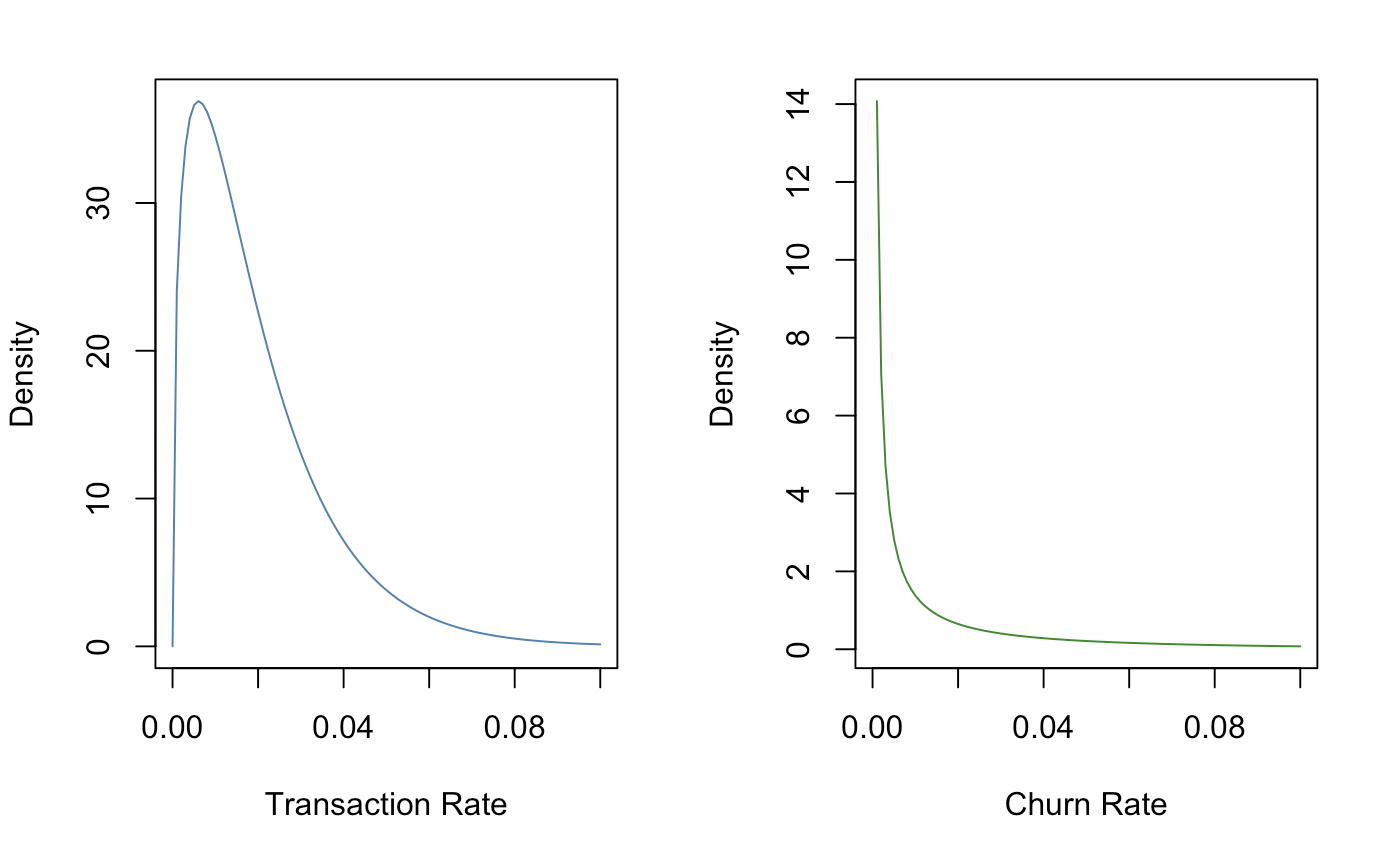
Also, if you were curious on finding the average value of transaction and churn rates, you can just divide the shape by the rate (parameter1/parameter2).
params[1]/params[2]
params[3]/params[4]
[1] 0.01977308
[1] 0.002110926
Of course, these are on the date grain, so it is quite obvious that we see some amazing performance on any given day. Now the expected purchase volume by year is given by using the pnbd.Expectation() function. Another note to make about the av_sale value is that this does not have to be conditional on the entire customer database. Since there are hierarchical patterns, the av_sale value can (probably should) be determined by customer segments.
pnbd.Expectation(params, t=365)*av_sale
# [1] 430.0663
The P-NBD model predicted that each customer’s expected purchase rate ‘should’ be higher. Which may go to show that the average historical performance was lower than what was distributionally typical. In terms of benchmarking, this could be important information!
Taking it even a step further, we can take specific customers and predict their purchase behavior.
customer_prediction <- function(CID) {
  pnbd.ConditionalExpectedTransactions(params,
                                       T.star = 365,
                                       cal.cbs[CID,'x'],
                                       cal.cbs[CID,'t.x'],
                                       cal.cbs[CID,'T.cal'])
}

preds <- as.character(clean.elog$cust) %>%
  sapply(function(x) customer_prediction(x)*av_sale)

data.frame("CID" = clean.elog$cust,"CLV" = preds) %>% head
    CID       CLV
1 12472  628.9267
2 12647  637.2641
3 12712 1008.6756
4 12712 1008.6756
5 12471 1676.7700
Voila! Now we have a CLV value assigned for each customer. Furthermore, if we wanted to predict customers that are not in this period, all we need to do is to estimate their parameters and stick it right in.
Cool right? Although the traditional method of CLV calculation isn’t necessarily inaccurate, being able to assign CLV values to each customer can be a powerful thing. For example, in any customer segmentation project, we SHOULD include any RFM statistics along with CLV. With the traditional method, the best you can do is break down CLV by group. If you go down to the customer grain we would lose the ‘average’ tendency. It just isn’t so stable. Oftentimes the right tool needs to be used for the right job!
Best of luck in your next analytics endeavors!