This may seem a little cynical..

Ted talks are so popular, “TED.com currently have over 2,500+ talks, with addition every single day. tedx - YouTube channel, there are currently a little over 100,000 videos with 9.3M subscribers” (TED.com). It’s surreal how demanded these “motivational” speakers are.
Our goal is to create our own speaker session by discovering which topics are the most popular. Of course, that is definitely not enough to create a business model, however we this will be some important research.
Here is our dataset of TED talks. It’s a rather annoyingly medium sized file (7MB), so don’t freak out if it doesn’t run well on disk.
Here are the libraries to use for today.
library("tidyverse")
library("glmnet")
library("plotly")
library("plotmo")
To figure out what type of analysis to run, let’s take a glimpse into our data (if you’re not interested in the data and just into how to run the model with the parameters, keep scrolling down).
ted <- read.csv('ted.csv', stringsAsFactors=FALSE) %>% as.tibble # same as read_csv
glimpse(ted)
## Observations: 2,550
## Variables: 17
## $ comments           <int> 4553, 265, 124, 200, 593, 672, 919, 46, 852, 900, 79, 55, 71, 242, 99, 325, 305, 8...
## $ description        <chr> "Sir Ken Robinson makes an entertaining and profoundly moving case for creating an...
## $ duration           <int> 1164, 977, 1286, 1116, 1190, 1305, 992, 1198, 1485, 1262, 1414, 1538, 1550, 527, 1...
## $ event              <chr> "TED2006", "TED2006", "TED2006", "TED2006", "TED2006", "TED2006", "TED2006", "TED2...
## $ film_date          <int> 1140825600, 1140825600, 1140739200, 1140912000, 1140566400, 1138838400, 1140739200...
## $ languages          <int> 60, 43, 26, 35, 48, 36, 31, 19, 32, 31, 27, 20, 24, 27, 25, 31, 32, 27, 22, 32, 27...
## $ main_speaker       <chr> "Ken Robinson", "Al Gore", "David Pogue", "Majora Carter", "Hans Rosling", "Tony R...
## $ name               <chr> "Ken Robinson: Do schools kill creativity?", "Al Gore: Averting the climate crisis...
## ...
Not bad on size. For us to figure out which explanatory variables will predict well, we will probably need to use some robust nonlinear regression. However, with this p of columns, we will definitely need to do some feature selection. In the past, we ran a stepwise regresssion. However, this time we can use a continuous method: LASSO.
Lasso is an acronym for Least Absolute Shrinkage and Selection Operator. Mathematically, Lasso is a regularization model that penalizes the number of features in a model in order to only keep the most important features.
brilliant. LASSO limits the absolute sum of coefficients in a regression model by shrinking the high coefficients (these will usually overfit anyways) and small coefficients to zero. In a sense, it is shrunk to reduce multicollinearity since these are more likely to be low signal to noise, increasing predictive power. It uses 2 parameters alpha and lambda.
- Alpha is the parameter which decides whether to minimize the Reduced Sum of squares or coefficient sum of squares. It usually takes values rom 0 to 1 where 0 is our ordinary least squares estimate, 0.5 is our ridge regression, and 1 is our elastic net. We will need to set this value on our own.
- Lambda is the shrinkage parameter. It is otherwise known as the penalty coefficient that increases with the number of our variables. To select, we search for the minimum lambda value after cross validating.
We won’t get deep into the math. If you are interested in learning, send me a message or check out Analytics Vidhya.
But how come a lasso over stepwise? In all honesty, stepwise is computationally heavy and annoying. With Lasso, you don’t need to utilize an arbitrary percentage # feature to keep, since some of those may not be informative. Furthermore, you lose significant interpretability in your model as it focuses on prediction. The motivation leading to stepwise regression is that you ahve a lot of potential predictors, but not enough data to estimate their coefficients in a meaningful way. Since the model is taken out of the constraint of ordinary least squares, we don’t need to worry about collinearity.
Alright, we are good to go.
The way we analyze the model will be to use predictor variables of comments, durations, number of speakers, tag data, and ratings data against our total viewership. I’ve manipulated the information so we will be able to run it straight away. If you’re curious about how the data was cleaned up, take a look at the code here.
# load the clean dataset.
paths <- "https://raw.githubusercontent.com/tykiww/projectpage/master/datasets/Ted/lasso_ready.csv"
lasso_part <- read_csv(paths)
Lasso in R only takes matrix X’s and a vector for the predictor. In python, you’ll have to standardize the x values as mu = 0 and sd = 1. However, R takes care of that for us. We’ll just stick it into their own matrices.
x <- model.matrix(views ~ ., data = lasso_part)[,-1]
y <- lasso_part$views
Now the formula is simple. All we need is to stick it in this line of code.
gmlnet(x,y,lambda)
Now to find the best lambda, we will need to cross validate using the lowest error. We will choose the root mean squared error to standardize on near values. There is always a better way. Actually, cv.glmnet already cross validates for you without having to loop anything. However, I am a little wary of this unsupervised technique, so we will compare our errors manually. Also, note that we could have chosen more values for lambda if we desired (more than just 200), however for the sake of validation we will keep it this way.
# Using cross validation to determine optimal lambda
k <- 3
set.seed(15)
possible_lambdas <- seq(0, 200, 1) # only up to 200

lambda_rpmses <- c()

for (l in possible_lambdas) {
  print(l/length(possible_lambdas)*100)
  rpmses <- rep(0, k)
  for (cv in 1:k) {
    train_rows <- sample.int(n = nrow(lasso_part), size = floor(.8 * nrow(lasso_part)), replace = F)
    lasso_model <- glmnet(x[train_rows,], y[train_rows], lambda = l)

    preds <- predict(lasso_model, s = l, newx = x[-train_rows,])

    rpmses[cv] <- sqrt(mean((preds - y[-train_rows])^2))
  }
  lambda_rpmses <- c(lambda_rpmses, mean(rpmses))
}
Let’s plot out our potential lambdas and their rpmses.
# Looking at potential lambda values and associated rpmse
a <- data.frame("lambda" = possible_lambdas, "rpmse" = lambda_rpmses) %>%
  ggplot(aes(lambda, rpmse)) +
  geom_point()

ggplotly(a)
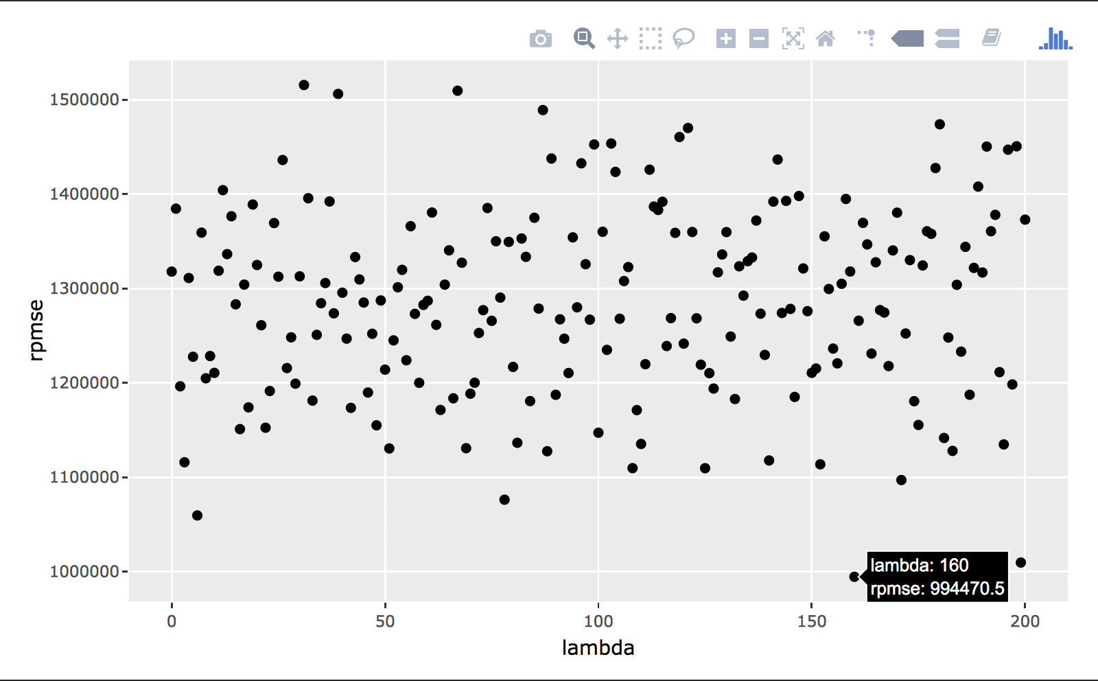
We notice here that the best lambda value is 160, minimizing our error at the optimal rate. We’ll stick that back in and view our most important coefficients.
# Getting the alpha that minimizes rpmse
best_lambda <- possible_lambdas[which.min(lambda_rpmses)]

# Fitting the model
lasso_model <- glmnet(x[train_rows,], y[train_rows], lambda = best_lambda)
With a lambda of 160 (log lambda of 5.075), here is what our variable trace chart will look like.
plot(cv.glmnet(x,y)$glmnet.fit,"lambda",label = TRUE)
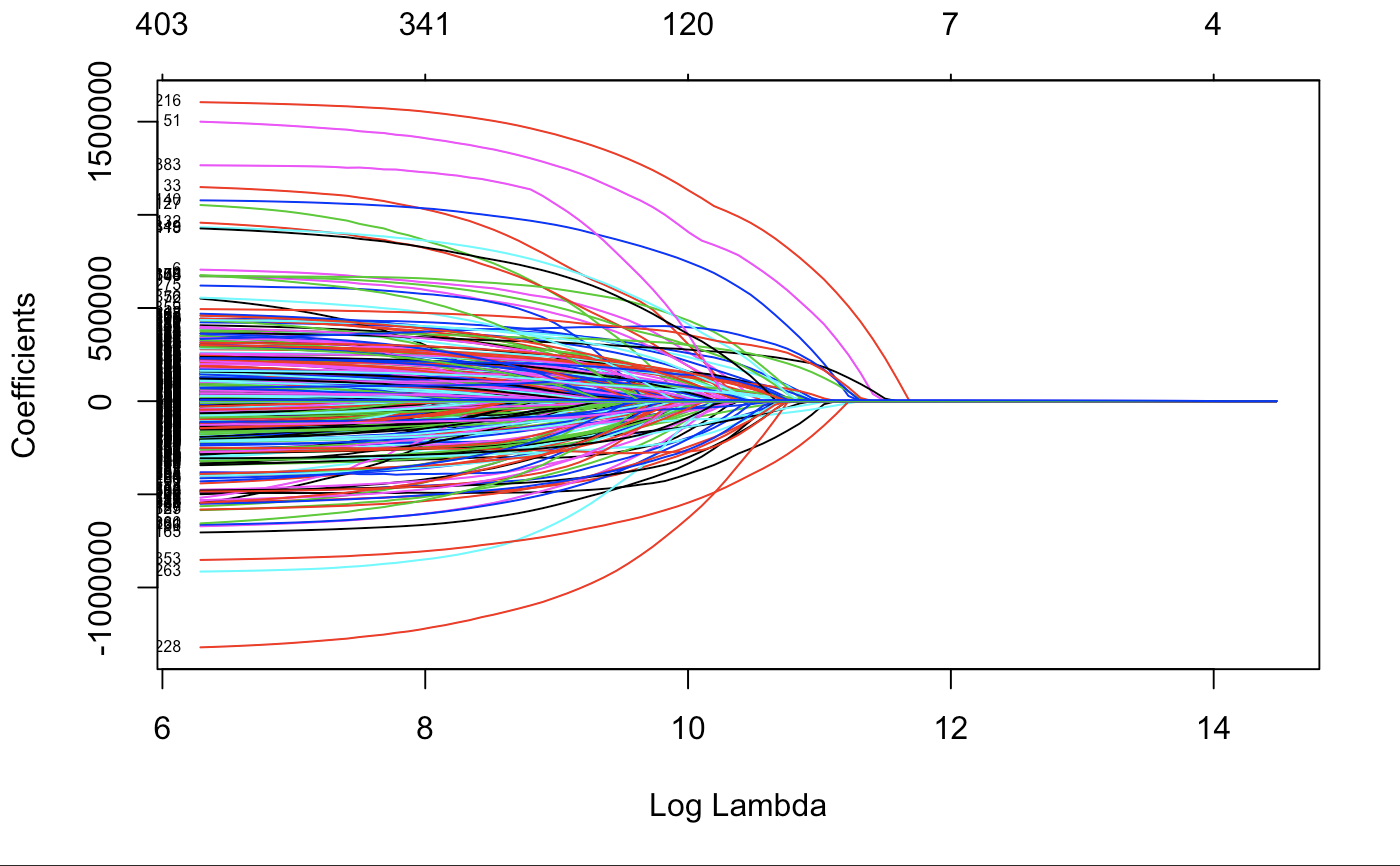
It is keeping many of the variables with only lambda of 200. However, we will see which ones go to 0 fastest.
Results
Now here is our most influential tags. (10 best or worst)
x1 <- rownames(coef(lasso_model))
x2 <- as.vector(coef(lasso_model))
det <- cbind("coefficient" = x1,"value" = abs(x2)) %>%
  as.tibble
des <- cbind("coefficient" = x1,"value" = x2) %>% as.tibble

# influential tags
arrange(det, .bygroup = desc(as.numeric(value))) %>%
  head(10)
## coefficient                  value
## `TAG_body language`TRUE	    1709814.80523373
## TAG_fashionTRUE	            1470516.24298873
## `TAG_TED Residency`TRUE	    1461828.39790206
## `TAG_augmented reality`TRUE	1407987.19606196
## TAG_memeTRUE	                1352322.74504519
## TAG_wunderkindTRUE	          1229587.96134256
## TAG_prisonTRUE	              1082654.5057984
## TAG_speechTRUE	              1047114.18347385
## TAG_statisticsTRUE	          1037541.56142934
## TAG_novelTRUE	              1026445.72865458
Here is our top 10 best tags that influence viewership.
# best 10 tags
arrange(des, .bygroup = desc(as.numeric(value))) %>%
  head(10)
## coefficient                  value
## `TAG_body language`TRUE	    1709814.80523373
## TAG_fashionTRUE	            1470516.24298873
## `TAG_TED Residency`TRUE	    1461828.39790206
## `TAG_augmented reality`TRUE	1407987.19606196
## TAG_wunderkindTRUE	          1229587.96134256
## TAG_prisonTRUE	              1082654.5057984
## TAG_speechTRUE	              1047114.18347385
## TAG_grammarTRUE	            969575.130343731
## TAG_cloudTRUE	              927640.200866753
## TAG_AddictionTRUE	          902238.558476863
Here is our worst 10 tags that influence viewership.
# worst 10 tags
arrange(des, .bygroup = as.numeric(value)) %>%
  head(10)
## coefficient                  value
## TAG_memeTRUE	                -1352322.74504519
## TAG_statisticsTRUE	          -1037541.56142934
## TAG_novelTRUE	              -1026445.72865458
## `TAG_human origins`TRUE	    -991317.23396853
## TAG_GoogleTRUE	              -952820.229984193
## TAG_IslamTRUE	              -883683.735178809
## TAG_miningTRUE	              -796222.535043558
## TAG_presentationTRUE	        -726388.416042411
## TAG_suicideTRUE	            -706981.54572895
## TAG_advertisingTRUE	        -705560.176234764
Finally, the tags that had no influence
# Useless tags.
subset(des,des$value==0)
## coefficient                  value
## TAG_AlzheimersTRUE	          0
## TAG_decisionmakingTRUE	      0
## TAG_goalsettingTRUE	        0
## TAG_newsTRUE	                0
## TAG_nonviolenceTRUE	        0
## TAG_opensourceTRUE       	  0
## TAG_statebuildingTRUE	      0
## `TAG_TED en Espaol`TRUE	    0
## TAG_TEDEdTRUE	              0
## TAG_testingTRUE	            0
So-according to our data-no one cares about alzheimers, memes seem to be deterring views, and people love learning about body language and fashion. Of course, we need to be more introspective about our interpretation. We have no idea which subset of population these views are coming from. Furthermore, with this many variables we are most likely overfitting. Next time, we should search for a better lambda value.
Great thing is that LASSO seeks to estimate the same coefficients as OLS maximum likelihood does. The model is the same, and the interpretation remains the same. The numerical values from LASSO will normally differ from those from OLS maximum likelihood, but if a sensible amount of penalization has been applied, the LASSO estimates will be closer to the true values than the OLS maximum likelihood estimates. If we are going to predict, we should be able to with our simple predict function.
Hope you enjoyed this small exercise.