The often incalculable volatility of the market makes investing a fearful avenue to approach. However, one method to vaguely estimate the enterprise value of our company and deduce potential earnings for a growing business.

I am no expert in financial modeling, but I know enough of some accepted techniques used as methods for valuation. One mentioned here, in the title, is the Discounted Cash Flow method. The discounted cash flow method allows an agent to deduce the net present value of the firm over a period of time. The model accounts for the sum of the cash flow forecasts over a period of time, divided by the compounding interest rate. The formula is given below.
## DCF = [CF1 / (1+r)^1] + [CF2 / (1+r)^2] + ... + [CFn / (1+r)^n]
- The summation goes from 1 -> n.
- r used here will be the discount rate (or the Weighted Average Cost of Capital if you were to finance a business).
- CF is known as the predicted cash flow per year.
- Cash flow MUST be > 1. As there will be a systematic error in calculation
- consider using the dividend discount model or deducing the ggm model if the company doesn’t pay dividends.
Now here is the challenge. Within the DCF context, the analyst is required to find a dependable net present value that approaches a true parameter. To control for this output, unfortunately, growth rates in future cash flows are expected to grow homogenously and the required rate of return or cost of capital remains fixed. Since we know that the values of cash growth and discount rates are not stagnant, we run into our dilemma.
There is no ‘one tool’ to figure this problem out, as we know from our friend George Box: “All models are wrong but some are useful”. We have to do our part to put our ingenuity to use, but what can we use? My means to accomplish this method here is to run a Monte Carlo to simulate unknown parameter estimates of tens of thousands of outcomes. The randomly sampled variables will vary the major model inputs of (1) cash flow growth rates and our (2) cost of capital discount rates. This is done in hopes to help us depict a better view of the possible ‘true’ NPV.
Yet, before we get ahead of ourselves let’s set up the model we are trying to run our MC with! Here are the functions that will run our calculations.
Our cash flow will be given by the gordon growth model. I made a quick function that compounds each years’ growth and gives us the terminal value and projected cash flows.
library(tidyverse)
GGM <- function(TTMFCF,LTGR,DR, n) {
  # TTMFCF: trailing twelve month Free cash flow (numeric)
  # LTGR: long term growth rate (vector of length n)
  # Overall growth for terminal year will be an average of the long term growth rate vector.
  # Discount Rate (WACC)
  # n for length of period.

  a <- TTMFCF
  b <- LTGR
  c <- DR
  d <- mean(LTGR)
  years <- c(a)

  for (i in 1:n) {
    years[i+1] <- years[i]*(1+b[i])
  }

  years[n+2] <-  years[n+1]*(1+d)/(c-d)
  tval <- years[n+2]
  CF <- years[2:(n+2)]

  list("Cash Flow" = CF, "Terminal Value" = tval)
}
We move on from here to create the function to calculate DCF. This will give us the NPV of any company as long as the cash flow, discount rate, and n are given.
DCF <- function(CF,DR,n) {
  a <- list()
  cash <- c()
  for (i in 1:n) {
    cash[i] <- CF[i]/((1+DR)^i)
  }
  cash[n+1] <- CF[n+1]/((1+DR)^(n))
  sum(cash)
}
We top this off by dividing our NPV by our outstanding share count to see if we make it past our cutoff value.
(dcf/outstd) > price
If we were to use a hypothetical situation (Apple) with fixed values, it would look a little like this:
price <- 191.33 # Apple stock price from bloomberg
TTMFCF <- 53726 # Made up Trailing FCF * 10^6
LTGR <- c(.01,-.02,.03,-.01,.01) # Guessing the long term growth rate for 5-year period.
DR <- 0.12 # Choosing a reasonable WACC of 12% (made up)
n <- 5 # number of years
outstd <- 861.74*10^6 # shares outstanding (10 million shares)


# calculate cash flow (should be vector)
CF <- GGM(TTMFCF,LTGR,DR,n)[[1]]
## [1] 54263.26 53177.99 54773.33 54225.60 54767.86 474025.25
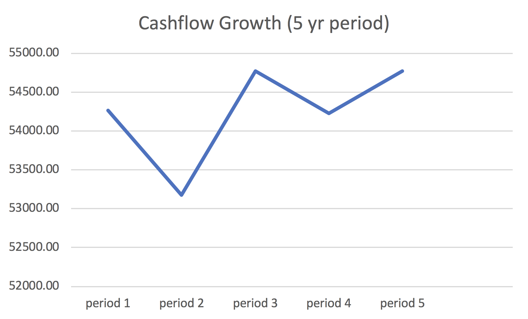
Above is the predicted cash flow per year with the terminal value attached at the end. Of course, remember that we made up the growth patterns and discount rate on a whim. We can’t predict for those without their information. That is what we’ll be doing a monte carlo with.
Below is our predicted stock price!
# use CF to figure out DCF
dcf <- DCF(CF,DR,n)*10^6

# Divide NPV by outstanding shares
dcf/outstd
## [1] 551023365875   # NPV
## [2] 538.8422       # predicted share.
The price of $538 is a 280% growth from what it is currently. With the amount of cash flow, fixed discount rate, and growth it’s certainlly not impossible (Consider the stock price of Amazon currently at 1,822.49).
Now that we are done with the setting up of our functions, we are going to expand this by running a monte carlo on both the discount rates and cash flow growth. Note here that we will need to set the seed twice to use the same random pattern for both DR and CF growth. We will use 100,000 iterations.
Let’s begin by using same data as our example from Apple. Our most up-to date information is pulled from both the apple website and zacks.com, giving us the following values we will need to forecast for the next 5 years.
- 8.7 Billion Shares Outstanding
- Stock Price (from bloomberg): 13.90 USD
- Trailing Free Cash Flow is $9,346
Let’s begin with the information we have.
price <- 191.33 # stock price
outstd <- 861.74*10^6 # shares outstanding (in 10 millions)
TTMFCF <- 53726 # Trailing twelve month free cash flow in *10^6
n <- 5 # period of projected cash flow.

# missing long term growth rate and discount rate
Now that we have our basic info, let’s move on to our iterations.
There are so many different ways to run a random sample, but here we will use the replicate() function sice we already have our function at hand. Unfortunately for us, more assumptions need to be made: Which bounds do we use for our replications (mean, standard deviation)? Do we assume normality?
We will suppose management has calculated historical averages on our parameters with a standard deviation of 1%. This assumption is given as year to year differences do affect the next year’s costs and growth, but tend not to change too notably. To make it easier on ourselves, let’s also assume normality.
- growth rate mean: 3%
- growth rate sd: 1%
- WACC mean: 14%
- WACC sd: 1%
We will first start with randomizing our gordon growth model. By embedding our function within the replicate statement, we make 100,000 replicates of our DR and growth rates. Our output is a histogram of the average cash flow amounts
set.seed(15)
reps <- 100000

rep.data <- reps %>%
  replicate(
    GGM(TTMFCF,LTGR = rnorm(5,mean = .03,sd = .01), n = 5, DR = rnorm(1,mean = .14, sd = .01)))

check <- sapply(rep.data[1,],mean)
hist(check)
mc.err <- quantile(check,c(.025,.975))
abline(v=mc.err,col='red')
##      2.5%    97.5%
##  127409.4 173481.3
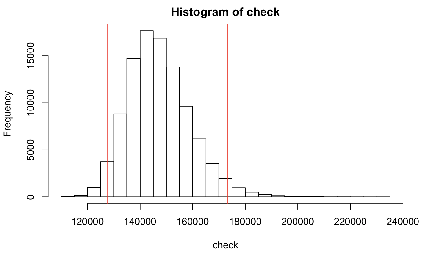
Here, we would expect the average cash flow to stay reasonably within the range of 127,000 and 173,000 as the company grows with a varying WACC (95% confidence). This seems to be a good sign.
Moving on to finding our DCF, we will once again set the seed at 15 to get matching discount rates and loop through our DCF() function.
set.seed(15)
DR <- replicate(10000,rnorm(1,mean = .14, sd = .01))
CF <- rep.data[1,]
DCF(CF[[189]],mean(DR),5)

stock <- c()
for (i in 1:reps) {
  stock[i] <- DCF(CF[[i]], DR = DR[1], n = 5)*10^6/outstd
}
hist(stock)
mc.err <- quantile(stock,c(.025,.975))
abline(v=mc.err,col='red')
##     2.5%    97.5%     mean
## 510.6132 676.6112 582.3326
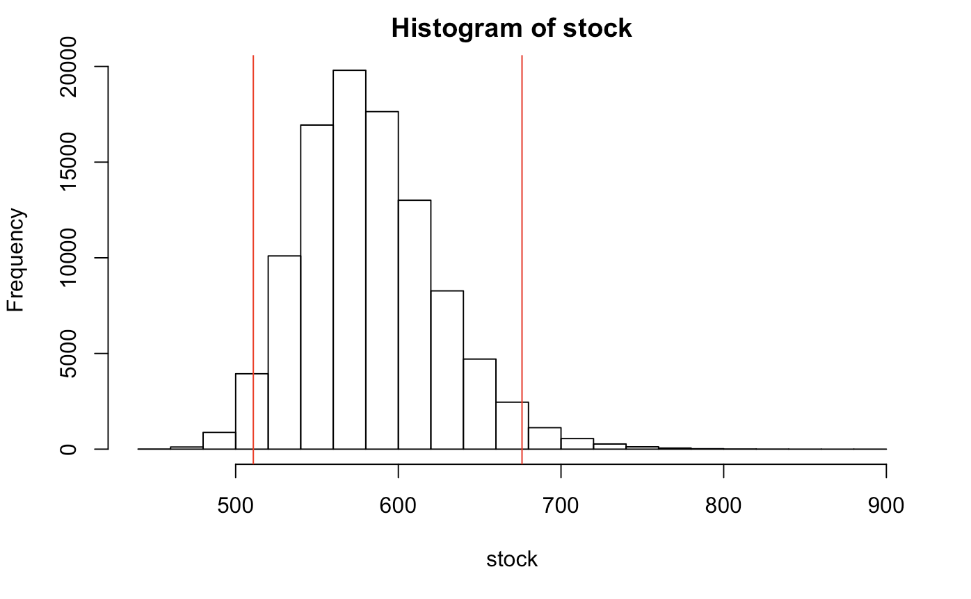
After accounting for monte carlo samples of 100,000 we can be 95% confident that the range of our fair equity value per share will be around $582.33 (95%CI: 510.61,676.61) as we account for variability in WACC and cash flow growth. Of course, we need to realize that this is should be dependent on the average performance of the WACC and long term growth estimated with informed decision. Yet, we realize here that, with continued growth, there is good reason to take a look into investing to this company.
Of course, we did throw in some garbage so with that we get some trashy results -those were the assumptions made as to the historical performance of Apple. Yet, we made sure to keep reasonable estimates that seem closely related to their past performance. Better data will yield better results.
Every company will be different. In many cases, DCF will not be the best predictor for growth as it does not take into account what happens to the cash flow (it stays within the company until management makes a decision). Executives may spend that cash on acquisitions, stock buybacks, new projects, or even bonuses. The cash flow just doesn’t reflect the full decision making process of the organization. Even with all other factors considered, our critical thinking will be the overall, most powerful, factor for success.