We oftentimes undermine the power that non-parametric methods have in predicting probabilities of outcomes. Sometimes, we just don’t have enough data to find out a confidence estimate and interval of an outcome. Other times, we lack information to perform accurate hypothesis tests of statistical significance. These situations usually lead to requiring augmentation models to figure out likelihood estimates of certain outcomes with the limited information!
Fortunately, we have the monte carlo method to give us a good gist. Monte carlo sampling is a technique that allows for estimates to follow a pattern of the law of large numbers, creating a central limit distribution. In other words, MC takes a random sample of certain events (parameter) over and over and over and over again to obtain numerical events from uncertainty. Monte Carlo sampling is very useful when determining confidence estimates from non-parametric distributions. As long as we are familiar with a ‘true’ proportion or a tendency of the estimate, we can create confidence estimates.

One type of monte carlo sampling is the bootstrap technique (this is something that briefly covered in a random forest models post in the past). Bootstrapping is one of the most useful procedures in determining confidence interval parameter estimates and is a sampling technique with replacement (replacement means, that every time an object is sampled, it is replaced back with the same probability of independent occurrence). This is especially useful when we have known/estimated probabilities of certain outcomes and we are testing with limited amounts of data. Bootstrapping has been known to be valuable in dealing with optimization when there may be heteroscedasticity (errors are not normally distributed) and distributional assumptions may not be met.
In short, it’s a ridiculously useful technique to create more data when we have just partial information. Well then, let’s take a look at some coding!
===================================
Case
You are a pest control sales agent looking to figure out how many doors you need to knock on, before having at least 1 potential customer (an individual that ‘at the least’ gives you their contact info). Let’s just say, that this event X is represented by a geometric distribution (n = 1,2,..100) with p = 0.2 for this particular area (a gross oversimplification).
If you were to knock on a total of 100 doors that day what is the average number of doors you must knock to reach a potential customer?
library(tidyverse)
This problem is rather simple. Since we are looking at the number of doors ‘until’ we reach a potential customer, we notice that this is geometric. To create our data, we will use rgeom() + 1. For a more precise simulation, we could use the actuarial package actuar using the given function: rztgeom(n, prob).
Model
To begin, we will initialize some parameters of interest. Just to note, taking about 100,000 samples is pretty much a standard. 10,000 may be okay, but the larger you have the better it is.
doors <- 100 # If we knocked on 100 doors that day.
p <- 0.2 # overall probability of getting in a house (not bad dude)
n_reps <- 100000 # monte carlo repetitions
Next, we will create a function to produce confidence intervals on each randomly generated set of values. This is separated into mean confidence intervals and proportion confidence intervals. Just to note, that these intervals are practically same. However, the proportion is different because it is a biased estimator. With enough samples, it is accurate up to 3 decimal points (since it’s a proportion).
ci <- function(x, prob = FALSE) {
  if (prob == TRUE) {
    mean(x) + c(-1, 0, 1) * qnorm(.975)* sqrt(mean(x)*(1-mean(x)/length(x))
  } else {
    vals <- confint(x) ; c(vals[1], mean(x), vals[2])
  }
}
Next is our model. As a brief explanation, we notice that we are replicating the sample of just 1 parameter over and over again. After sampling our data from our geometric, we are performing confidence intervals on all the data. These intervals are unlisted and created into tables. We should have 100,000 confidence intervals!
set.seed(15)

replicate(n_reps,{
    data <- rgeom(doors,p)+1
    data %>% ci(FALSE)
  }) %>% unlist %>% t %>%
  as_tibble -> sims

# Without piping..

    ### temp <- replicate(n_reps, {
    ###     data <- rgeom(doors,p)+1
    ###     ci(data, FALSE)
    ###   })
    ###
    ### temps <- t(unlist(temp))
    ### sims <- as_tibble(temps)
Now, technically, that was it! Let’s plot the distribution we have calculated and see how we are doing.
ci(unlist(sims[,2]), FALSE)
hist(unlist(sims[,2]))
## 4.998482 5.001254 5.004026
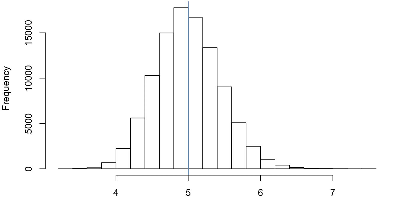
We see a rather normal plot of the number of times it takes to get in a door ~5 doors until a sale (not bad!)
If we were curious the probability of times we would have to knock on 6 doors or more, all we do is take the average of a boolean comparison.
mean(unlist(sims[,2]) > 6)
## 0.01636
That’s pretty impressive! If you were to go knock on doors, you 9/10 times you would get a sale before hitting 6-7 doors.
Assessing performance
Now, this is only in the case of having a true parameter of interest. As you noticed the many confidence intervals we generated with the replicate() function, our confidence intervals will not always capture the true mean. However, if we have a good enough model, all of our confidence intervals should contain the true value 95% of the time. Let’s take a look.
interval <- dplyr::select(sims,-2)
true_mean <- 1/p
mean(interval[1] < true_mean & true_mean < interval[2])
## 0.9425
For the geometric distribution, the true probability is 1/p. By sticking that into our comparison, we get about 94.25%. This confirms that we haven’t done our model incorrectly!
Now you’re happy, and the pest agency is happy. Everybody is happy. You’ll know how well you are progressing as you move forward!