The power of Regression predictions: How do you take into account multiple predictors and encapsulate it into one number?
Many times, people think that prediction in regression is solely used for guessing the future outcomes given a test dataset. However, this is farther from the truth. By the way, why are psychic mediums with a crystal ball always depicted as a woman?

Really quick, let’s decompose what a regression algorithm is trying to tell us.
\[y = \beta_{1}x_{1} + \beta_{2}x_{2} + ...+ \beta_{n}x_{n} +\epsilon\]So, here is our standard equation of a multivariate regression. We see that each $\beta$ corresponds to a covariate and its effect on the overall outcome. The overall product $y$ encompasses all the observed effects with an error term $\epsilon$.
Now what does that tell us?
That the term y is the sum total of all the effects and its magnitude with some variability. This means, if we create a model that incorporates a set of statistically significant covariates we can piece together a puzzle for what $y$ would actually look like with or without a certain $\beta$. Isn’t that crazy? In this way, we can actually see with our own eyes what our regression predictors are doing for us. Keep in mind that this intuition holds for any method of error minimization (normal equation, gradient descent, etc.).
Let’s give this thought a try by applying it in two scenarios. The data is loaded below for our use.
library(tidyverse, quietly = TRUE)
url <- "https://raw.githubusercontent.com/tykiww/projectpage/master/datasets/marketing_kaggle/retailmarket.csv"
dataset <- read_csv(url, skip_empty_rows = TRUE)
dataset <- select(dataset,-Age, -OwnHome,-Married, -History) # just for simplicity.
skimr::skim(dataset)
## Skim summary statistics
##  n obs: 1000
##  n variables: 6
##
## -- Variable type:character -----------------------------------------------------
##  variable missing complete    n min max empty n_unique
##    Gender       0     1000 1000   4   6     0        2
##  Location       0     1000 1000   3   5     0        2
##
## -- Variable type:numeric -------------------------------------------------------
##     variable missing complete    n     mean       sd p0      p25     p50      p75   p100     hist
##  AmountSpent       6      994 1000  1218.19   961.85  0   490.25   962.5  1688.75   6217 ▇▆▃▂▁▁▁▁
##     Catalogs       0     1000 1000    14.68     6.62  6     6       12      18        24 ▇▁▇▁▁▆▁▆
##     Children       0     1000 1000     0.93     1.05  0     0        1       2         3 ▇▁▅▁▁▂▁▂
##       Salary       0     1000 1000 55916.6  30748.39  0 29200    53700   76925    168800 ▆▆▇▇▃▂▁▁
Utility
Now how is this useful?
1) Filling in Missing data
2) Lego puzzles
Let’s go through each of these examples. They’re really simple.
Filling in Missing Data
In our dataset above, we have some spendings data of individuals. Not sure where or what its from, but seems useful. In the brief skim above, we notice 6 rows of missing data in our amount spent variable. IF we have good enough predictors, it is possible to fill in missing data.
missings <- dataset[is.na(dataset$AmountSpent),-6]
training <- dataset[!is.na(dataset$AmountSpent),]
(lmob <- lm(AmountSpent ~ ., data = training)) %>% summary
## Call:
## lm(formula = AmountSpent ~ ., data = training)
##
## Residuals:
##      Min       1Q   Median       3Q      Max
## -1725.55  -335.07   -34.31   227.69  2873.19
##
## Coefficients:
##               Estimate Std. Error t value Pr(>|t|)
## (Intercept) -5.260e+02  5.069e+01 -10.377   <2e-16 ***
## GenderMale  -4.191e+01  3.410e+01  -1.229    0.219
## LocationFar  5.148e+02  3.641e+01  14.140   <2e-16 ***
## Salary       2.103e-02  5.627e-04  37.376   <2e-16 ***
## Children    -2.040e+02  1.586e+01 -12.864   <2e-16 ***
## Catalogs     4.261e+01  2.555e+00  16.674   <2e-16 ***
## ---
## Signif. codes:  0 ‘***’ 0.001 ‘**’ 0.01 ‘*’ 0.05 ‘.’ 0.1 ‘ ’ 1
##
## Residual standard error: 515 on 988 degrees of freedom
## Multiple R-squared:  0.7147,	Adjusted R-squared:  0.7133
## F-statistic: 495.1 on 5 and 988 DF,  p-value: < 2.2e-16
It looks like almost all of the predictors are fairly strong estimates. Our R-Squared of .71 isn’t ideal but lets us know that we have good predictability. If we decide to spit back into our model, we can easily retrieve the missing data.
predict(lmob,newdata = missings)
##          1         2         3         4         5         6
##  -115.2360  810.2317  122.0629 2137.6427  208.3054 -438.5349
Of course, it doesn’t always turn out the way we would like it to be (I’m sure these customers aren’t giving away money). We can always tweak or handle these situations by omitting insignificant variables and using transformations.
lmob <- lm(log(AmountSpent + 1) ~ .-Gender, data = training) # there is a 0 in there (+1)
(preds <- predict(lmob,newdata = missings) %>% exp - 1)
dataset$AmountSpent[is.na(dataset$AmountSpent)] <- preds # Insert predicted values.
##         1         2         3         4         5         6
##  216.5663  468.5093  284.7971 1870.2489  288.9244  165.5069
I feel much more confident with these estimates. The standard errors are lower (.466), the predictability is higher (.743) and no negatives.
This is just a sidenote –
If you happen to be too lazy, you’re welcome to just use the missForest package to impute data using random Forests. Your prediction estimates will likely be closer and it will be less of a hassle.
library(missForest)
dataset <- missForest(dataset)
Lego Puzzles
Take for example a persuasive case you are trying to make of implementing a certain procedure. Can you prove something so intuition clicks?
You’re trying to market an ad and you are trying to set a theme. Your team looks vaguely at your regression summary and notices that Location seems to have a high, positive, significant coefficient. “Great, we’ll decrease marketing spend for local customers and look wider!” However, you stop and think at whether or not that is the best decision.
lmo <- lm(AmountSpent ~ Gender + Salary + Children + Location, dataset)

# Specify vector: 0.5 for mixed gender(jk median pay btwn male/female); 1 for far and intercept
element <- c(1, 0.5,median(dataset$Salary), median(dataset$Children), 1)

# Element-wise multiplication with coefficients
sumob <- element * lmo$coefficients

# Total Typical pay
(typical <- sum(sumob))
## [1] 1570.865
If the typical “far” customer brings in around 1570 dollars, Holding all else constant at a typical value, the percentage contribution of just the far customer amounts to..
t(cbind("Contribution"= round(sumob, digits = 2),"Percent"=round(sumob/typical*100, 2)))
barplot(sumob/typical, col = c("forest green"))
##              (Intercept) GenderMale  Salary Children LocationFar
## Contribution        8.24     -13.92 1216.33  -234.97      595.17
## Percent             0.52      -0.89   77.43   -14.96       37.89
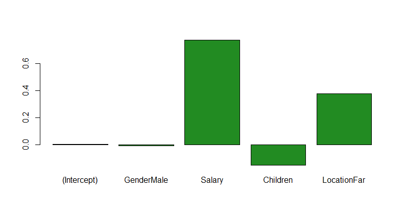
Yes, it seems like Location does play a large part in the total spend. 37%! However, there is a better power play. 77% ($1216) of the amount spent contributes to majority of that 1570 dollars EVEN AFTER CONSIDERING A FAR LOCATION. Now we can readjust by focusing more on the higher income individuals.
We can see how what we did earlier was just like fitting a puzzle (or legos). We can see the constituents of a regression model and really dive deep into understanding how to squeeze the utility out of it.
Another important aspect of this calculation is the fact that we are using the coefficients to inform the meaning of the prediction. Take for example these three columns in the following matrix.
mod1 <- lm(log(AmountSpent+1) ~ Catalogs + Salary + Children + Location, dataset) # included transformation to give more meaning to matrix below.
mod2 <- lm(AmountSpent ~ Location + Children, dataset)

cbind(
  "Real Data" = dataset$AmountSpent,
  "Full Model" = round(exp(predict(mod1))-1),
  "Part Model" = round(predict(mod2))
) %>% head
##   Real Data Full Model Part Model
## 1       755        865       1793
## 2      1318        791       1252
## 3       296        482       1252
## 4      2436       1564       1044
## 5      1304       1120       1252
## 6       495        408       1252
The real data is the amount of spend taking into account all possible values and interactions of values. The Full Model is the predicted amount taking into account Location, Salary, Children, and Catalog. However, the Part Model only takes into account Location and Children. In other words, there is much more meaning applied to the Full Model compred to the Part Model. That column actually identifies a revenue considered for the data we have.
Now, even if gender isn’t so statistically significant in our regression we can look at predicted spend based on gender differences.
mat <- data.frame("Gender" = dataset$Gender,"Pred_Spend" = exp(predict(mod1))-1)
aggregate(mat$Pred_Spend, by = list(mat$Gender),median)
## Female	704
## Male	1216
Does this matter in terms of ROI? Maybe? Depends on your strategy and product. We are able to glean a bit more information because this predicted number considers the variables we have at least controlled for.
In summary, there is way more we can do by understanding our regressions. Rgeression predictions do their best to take into account dataset covariates to help inform what our likely value will be whether it is through imputing missing data, or taking apart the most important variables. Being able to understand what these covariates mean in the bigger picture can potentially add tremendous value to your strategic decision making.