How in the world will we rid of this awful curse?

High dimension data is difficult to deal with, and I’ll show you why. This post explains why it is so important to have concise information.

Consider the following plots:

library(plot3D)
x = 1:10
y = exp(x)
z = log(x)
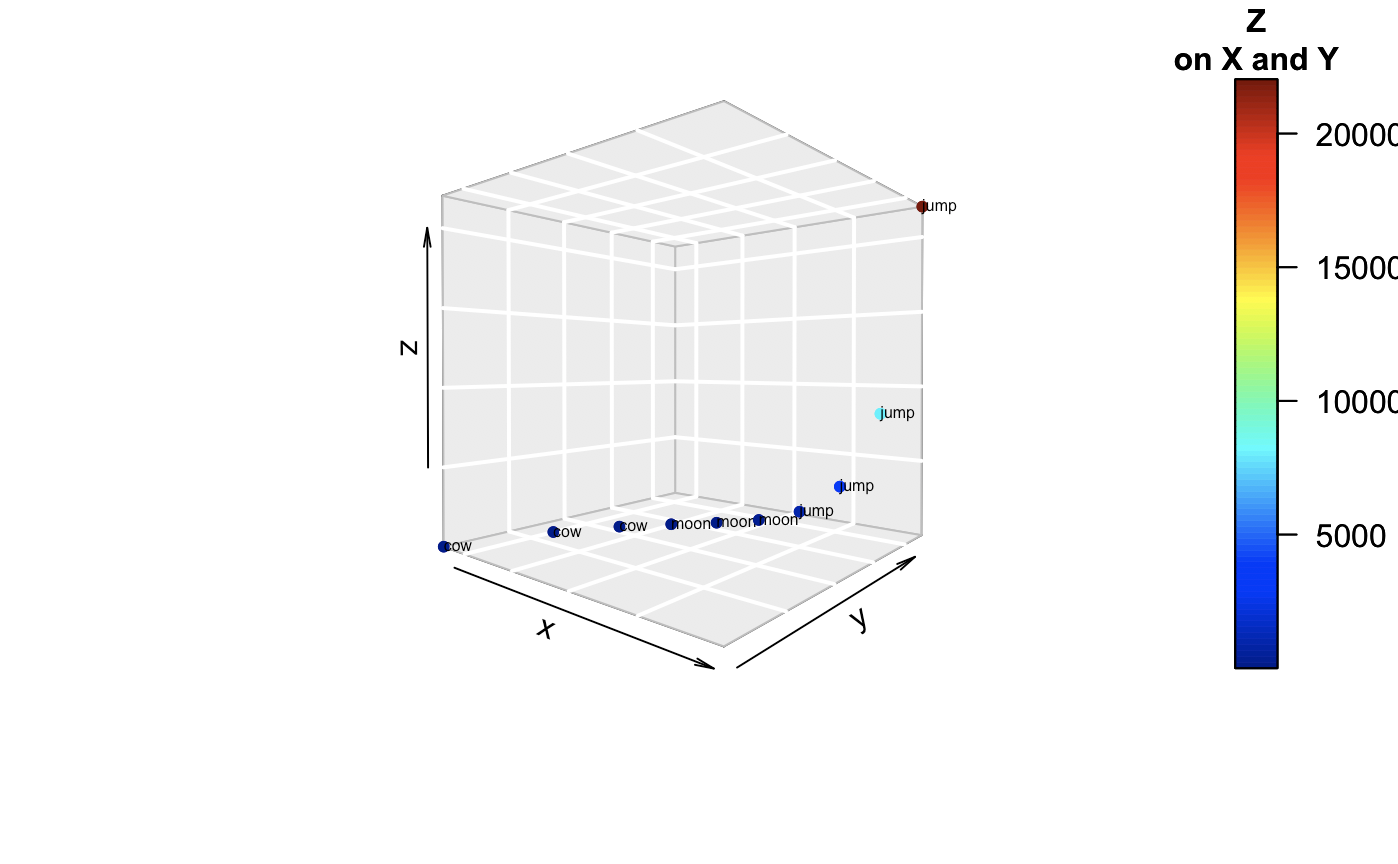
d = as.factor(c(rep("cow",3),
      rep("moon",3),
      rep("jump",4)))

par(mfrow = c(1,2))
plot(x,rep(0,10), col = "steel blue",
     pch = 20, cex = 1, xlab = "x", 
     ylab = "",yaxt = "n")

plot(x, y, col = "steel blue", pch = 20, 
     cex = 1, xlab = 'x', ylab = 'y')
par(mfrow = c(1,1))

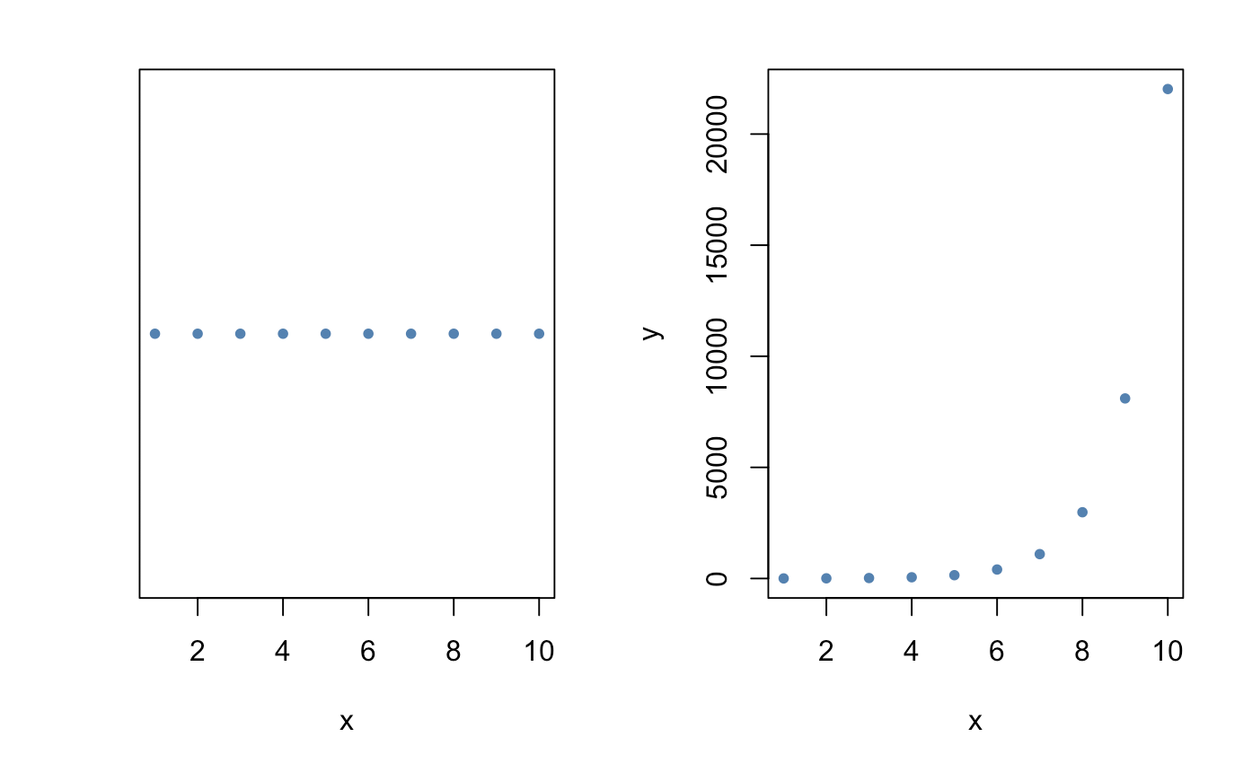
As many of you already understand, this is a 1 and 2-dimensional plot where we have either an x and a y or both. With just 2 axes, figuring out locality is easy. Just point and click.

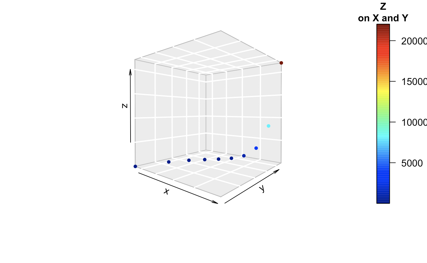
Now what if we increase the number of dimensions?

scatter3D(x, z, y, clab = c("Z", "on X and Y"), 
          phi = .5, bty = "g", pch = 20, cex = 1)
scatter3D(x, z, y, clab = c("Z", "on X and Y"), 
          phi = .5, bty = "g", pch = 20, cex = 1)
text3D(x, z, y,  labels = d,
        add = TRUE, colkey = FALSE, cex = 0.5)

Now, 3 can be done pretty well. We see that x, y, and z are all collinear to each other in some way. There is some model relationship that can be explicitly be observed here.

How about if we get into the 4th dimension. What do we do? Now we can’t really visualize, simply, another orthogonal plane. We’ll try another method. Some put hyperplanes or ellipses to show meaningful groups. Here we have simple text.

Beyond this, things get tricky. As you notice, higher dimensional objects just have much more ‘volume’. Having 4 dimensions takes up more in the latent space than a simple 1 dimension x. Now, think about a 10-dimensional object! The space will be filled up and results in a phenomenon that throws intuitive distancing. Everything starts looking closer and closer together, thus conflating the “difference” between objects.

If that doesn’t make too much sense to you, think about it this way. Let’s compare a biological male and a biological female (treading lightly here). For every same characteristic, we would label a 0 and for every different characteristic we will denote the difference of a 1. In the end, if we average up the total difference, we should get a number as close to 1 (different) as possible.

# bone structure, genitals, hormone balance,  ...(n)
[1, 1, 1,...]/n

We clearly know that they are differences in sex. However, when we start counting the presence of certain obvious aspects (eyes, nose, mouth, fingernails, toes..), the average distance between the two start to get closer and closer.

# bone structure, genitals, hormone, eyes, mouth, fingers, toes, eyelashes, ...(n)
[1, 1, 1, 0, 0, 0, 0, 0]/n

Although there may be obvious differences, having excess information makes the relative distance between the two groups closer. In the end, men and women might just end up being 99.99% similar to men if we aren’t careful in choosing the correct ‘dimensions’ to compare.

There are many more reasons why a higher dimensional space is not as appealing. However, learning in-depth methods to measure dimensional space can get extremely complicated.

So, what can you do?

There are a plethora of methods to tackle these problems: Penalized regressions, forward/backward selection, feature importance with random forests, principal component analysis, autoencoders, feature vectors, genetic algorithms, stochastic embeddings, variance/correlation filters, and … The list goes on.

The reason for why there are so many methods to solve this problem is a testament to the various types of data. You just have to test for the right fit. Now, at least with this basic understanding, we can confidently stroll into our future analytics projects.